What is Financial Modeling in Excel?
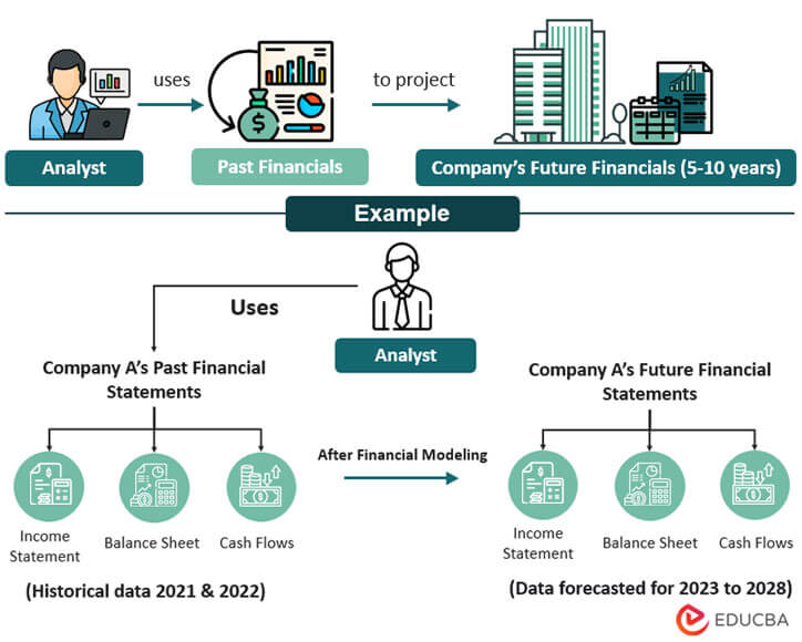
Financial modeling in Excel means using a company’s current and past financial data, well-researched assumptions, and Excel formulas to project (predict) all the numbers from its income statement, Balance Sheet, and cash flow statement for the next 5 to 10 years.
Financial analysts, accountants, investment bankers, and other professionals use it to make informed decisions about:
- Whether to invest in a company,
- Evaluate its potential for mergers and acquisitions,
- Determine fundraising options for the company,
- Assess its current and future risks,
- Predict its future financial performance.
While financial modeling skills are essential for analysis and forecasting, accounting professionals also need operational tools to manage their day-to-day practice. Specialized practice management platforms like Uku help accounting firms combine client relationship management, time tracking, and workflow coordination alongside their financial modeling work, allowing accountants to focus on analysis while the software handles project coordination and client communication.
However, mastering financial modeling isn’t a walk in the park. It requires a firm grasp of accounting principles, financial statements, and the company’s market conditions. You will also need reliable data sources and assumptions, for which you must be good at analysis and research.
Therefore, we bring you this guide that offers a practical approach to financial modeling in Excel. Professionals looking to master these practical skills often enroll in a financial modeling course to gain structured, hands-on training in Excel-based forecasting and valuation.
In this guide, we will teach you to create a fully integrated financial model in Excel for Apple Inc.
We will use Apple’s historical data from 2019 to 2023 and create projections for 2024 to 2028. Once you create this model by following the steps given below, you can create a financial model in Excel for any other firm, too.
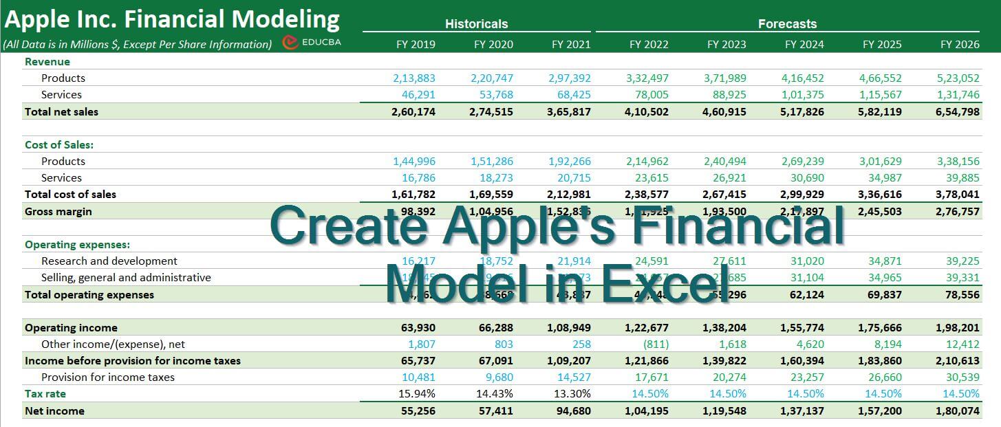
(Image Credit: EDUCBA Financial Modeling Course)
We have updated Apple’s financial model in 2024, as shown in the image below.
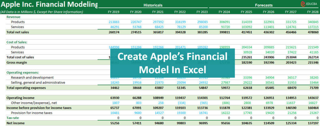
(Image Credit: EDUCBA’s Financial Modeling in Excel Training 2024)
Introduction to Creating a Financial Model in Excel
To help you get started, we have 2 free financial model templates of Apple Inc. One is the solution file, and the other one is without the solution, so you can practice on your own.
Disclaimer: Please note that Apple’s Financial Model in Excel is for educational purposes only. EDUCBA does not provide any buy or sell recommendations to investors or any other stakeholders.
Now, before we create a practical financial model in Excel, here are a few resources you can review to gain more theoretical knowledge of the concepts.
- How to Color-Code My Financial Model?
- Learn Financial Modeling in 15 Days
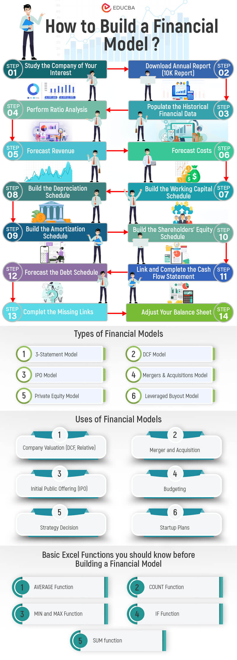
- Types of Financial Models
- What Financial Modeling Tools Can I Use?
How to Create a Financial Model in Excel? – Step-by-Step Guide
Make sure to have the “With Solution” template open while reading these steps.
- Download the Annual Report (10-K Report)
- Populate the Historical Financial Data
- Perform Ratio Analysis
- Forecast Revenue
- Forecast Costs
- Build the Working Capital Schedule
- Build the Depreciation Schedule
- Build the Amortization Schedule
- Build the Shareholders’ Equity Schedule
- Link and Complete the Cash Flow Statement
- Forecast the Debt Schedule
- Complete the Missing Links: Tax & Net Income
- Complete the Balance Sheet
Here is a detailed step-by-step explanation for making with financial modeling in Excel.
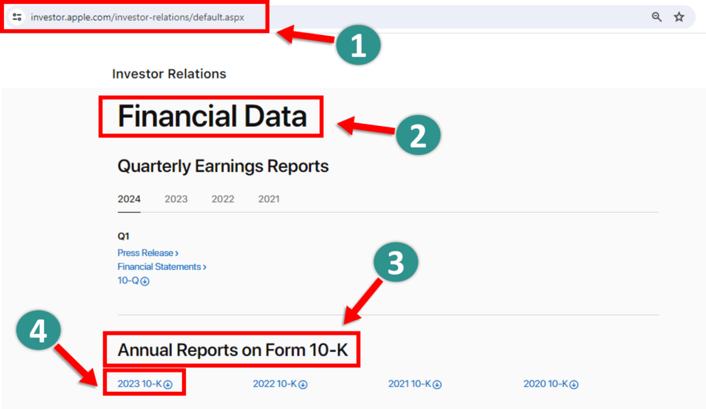
Step #1: Download Apple’s Annual Report (10-K Report)
The first thing we need to do is download Apple’s annual report from its official website. Here’s how you can do it:
- Go to Apple’s official website.
- Look for the “Investor Relations” section, which you can usually find in the header or footer of the website.
- Find the section where annual reports or 10-K reports are.
- Download the most recent ones. In our case, it’s the 2023 10-K.
Step #2: Populate the Historical Financial Data
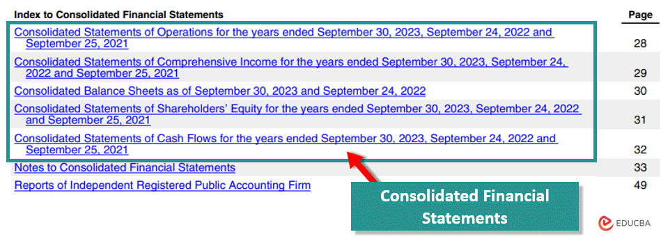
Apple’s historical data (2019 to 2023) is present in three Consolidated Financial Statements in its 10-K report:
- Consolidated Income Statment
- Consolidated Balance Sheet
- Consolidated Cash Flow Statement
Therefore, after downloading the 10-K report, search for “Consolidated Financial Statements” (FIND shortcut: Ctrl + F). This will take you to a section where you can view the company’s consolidated financial statements.
Important:
We only use the ‘Consolidated Financial Statements’ for data collection, as they give us a comprehensive view of the company’s financial situation. Don’t refer to the ‘Standalone Financial Statements’ as they only provide information about the company’s individual entities/subsidiaries, not the entire company.
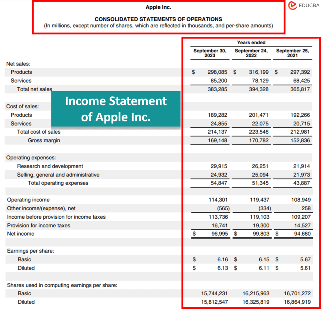
This is how Apple’s Consolidated Income Statement is present in its 10-K Report.
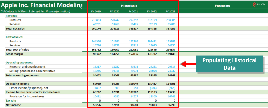
The next step is to populate all historical data from the 10-K report into Excel:
⫸ We have already done this for you. We have populated five years of historical data of Apple Inc. in the Income Statement tab, Balance Sheet tab, and Cash Flow Statement tab of an Excel sheet (Without Solution Template).
Step #3: Perform Ratio Analysis
Ratio analysis will help us understand how well Apple Inc. is performing.
We will be using vertical ratio analysis to create Apple’s financial model. Therefore, before calculating Apple’s ratios, you must know what is horizontal and vertical ratio analysis.
➔ Vertical ratio analysis involves comparing different line items on the financial statement for a single accounting period. For example, dividing Apple Inc.’s current assets and current liabilities for the year 2023 is a vertical ratio analysis.
➔ Horizontal ratio analysis compares any one financial parameter of a company over multiple years. For example, we can compare Apple Inc.’s revenue from 2019 to 2023 to understand its increase or decrease compared to the previous year. Similarly, we can compare other items like Research and development costs and see how much they have increased or decreased in percentage terms.
Now, let’s calculate some important ratios of Apple Inc.
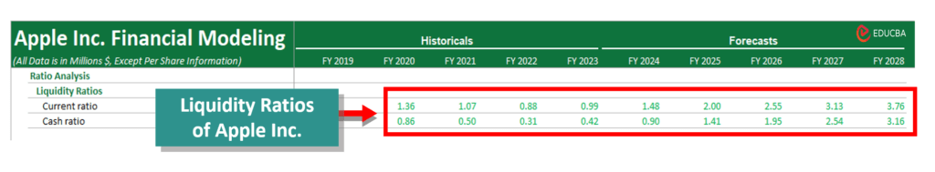
1. Calculate the Liquidity Ratios of Apple
Liquidity ratios show if a company has enough money to pay what it owes (debts and liabilities) in the short term (less than 12 months). A higher liquidity ratio means that the company has more than enough financial reserves and can easily cover what it owes.
Here are the most common liquidity ratios:
- Current Ratio= Current Assets / Current Liabilities
- Cash Ratio= Cash & Cash Equivalents / Current Liabilities
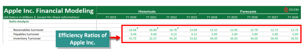
2. Calculate the Efficiency Ratios of Apple
Now, let’s move on to calculating the efficiency ratios of Apple. Efficiency ratios help us determine how effectively a business uses its available resources or turns its inventories into cash. We can also call them turnover ratios.
Here are some of the common efficiency ratios we can calculate:
- Receivables Turnover Ratio= Sales / Accounts Receivable
- Inventory Turnover Ratio= COGS / Average Inventories
- Payable Turnover Ratio= COGS / Accounts Payable
- Asset Turnover Ratio= Sales / Total Assets
- Equity Turnover Ratio= Sales / Total Equity
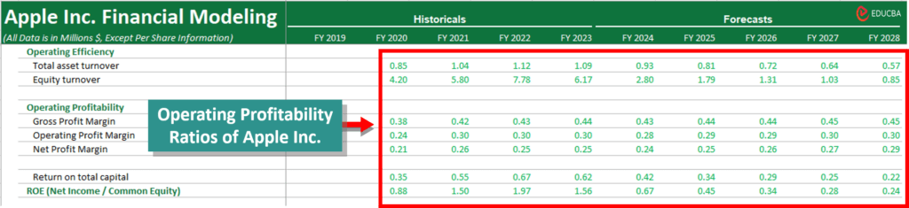
3. Calculate the Operating Profitability Ratios of Apple
Next, let’s calculate Apple’s operating profitability ratios. Profitability ratios help us evaluate the company’s ability to make money and generate adequate profits. Here are some of the common operating profitability ratios we can calculate:
- Gross Margin= (Sales – COGS) / Sales
- Operating Profit Margin = EBIT / Sales
- Net Margin= Net Income / Sales
- Return on Total Asset (ROA)= EBIT / Total Assets
- Return on Total Equity (ROE)= Net Income / Total Equity
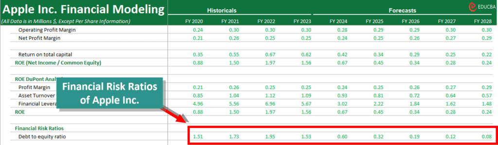
4. Calculate the Financial Risk Ratios of Apple
We use financial risk ratios to see if a business can meet its long-term obligations. For this, we compare the company’s level of debt to its assets or equity.
The most common financial risk ratios are:
- Debt-To-Equity Ratio= Total Debt / Total Equity
- Debt Ratio= Total Debt / Total Assets
Step #4: Forecast Revenue
Alright, let’s move on to the next step, i.e., forecasting Apple’s revenue. As a financial analyst, it’s important to spend extra time figuring out the best way to predict revenue. When choosing a method to predict revenue, you need to consider the type of company, its sector, and the information you have about it.
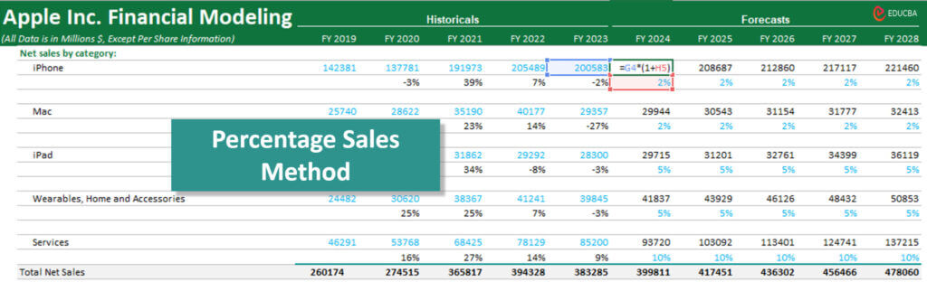
For forecasting Apple’s revenue, we will be using the segment-wise method. This method works well for companies with many different products or businesses. In this case, we first figure out how much each part of the company will make, then add it to get the total revenue.
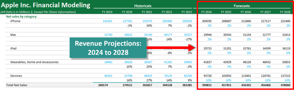
Here’s how:
- In Apple’s 10-K report or annual report, we will look at its products and services (like iPhones, Macs,iPads, Wearables, Home and Accessories, and Services).
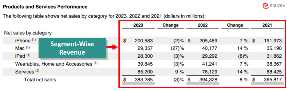
(Apple Inc. 10-K Report 2023, Page no 22)
- Once we have identified the products, we determine the year-over-year growth for each product segment using the percentage of sales method.
- After that, we add up individual segment revenues to get the total revenue forecast. This will give us a good idea of how much money Apple is expected to make from FY 2024 to FY 2028.
Here is the revenue forecast for Apple from FY 2024 to FY 2028.
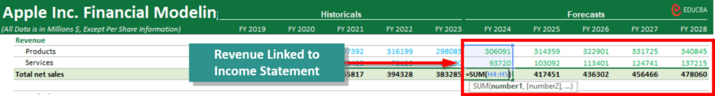
After forecasting the revenue numbers, we need to link them to the Income Statement.
Apart from the segment-wise method, there are a few other methods you can use to forecast revenue.
A) Geography-wise Revenue: It is useful for companies with offices in different countries like Microsoft, Coca-Cola, Procter & Gamble, and Nestle.
B) Revenue by Store Count: It is useful for companies that have multiple stores like Walmart, and Starbucks.
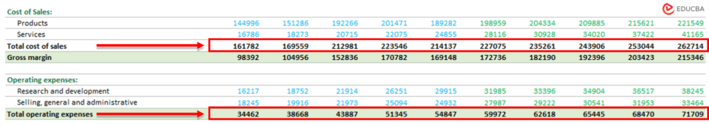
Step #5: Forecast Costs
After forecasting how much money a company will make in the future (revenue), we will now estimate how much it will spend (costs).
One way to forecast costs is called the vertical analysis approach. Here, we take a specific cost (like the cost of making “Product XYZ”) and divide it by the sales of that product for a year. This gives us the cost margin percentage, showing the portion of sales money used to cover the cost.
To predict how much that cost will be, you basically look at historical cost margins to estimate future-year margins. For example, Apple’s product cost was 64% of sales in 2022 and 63% in 2023. Based on this trend, we will assume it will be 65% for the projected years (FY 2024 to FY 2028).
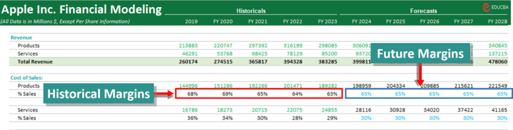
Now, using this margin (65%), we will find the product’s actual costs. We will multiply projected sales for a year ($3,06,091 Million) by 65% to get the product cost for that year ($1,98,959 Million).
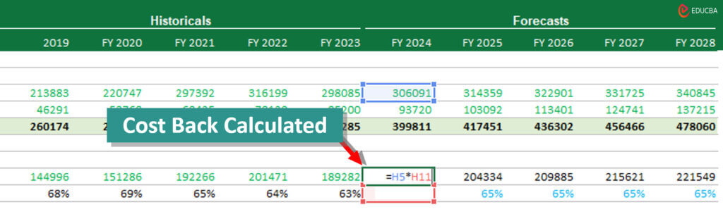
But that’s not all the costs. There are other expenses we need to consider too. So, we calculate the remaining costs and add them to the product cost to get the total operating expenses for the year. After that, we link these costs to our income statement to see how our company is doing financially.
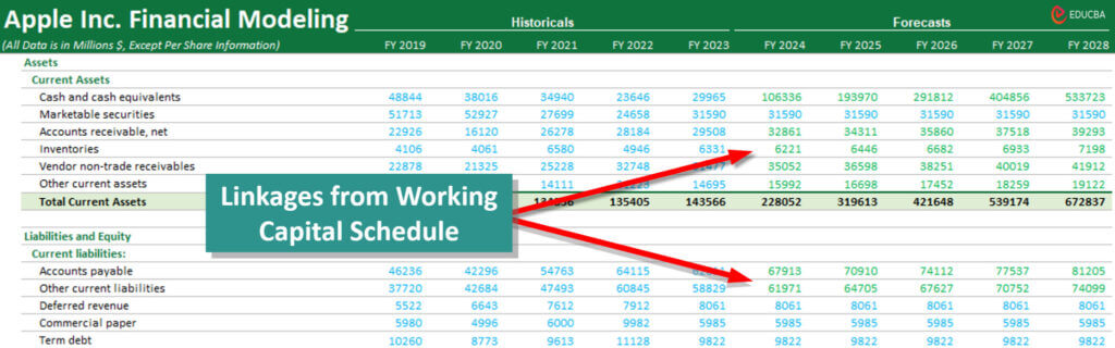
Step #6: Building the Working Capital Schedule
Follow these steps to create the working capital schedule:
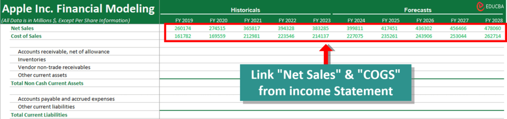
- First, link the Net Sales and COGS from the Income statement to the working capital schedule.
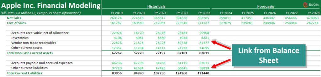
- Next, link the historical balance sheet data to the working capital.
- Now, let us calculate the historical ratios, like accounts receivable turnover, inventory turnover, and accounts payable turnover. Then, we can make assumptions about how these ratios will change in the future.
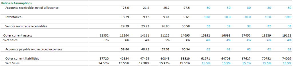
- Once we have our assumptions, we will calculate the future working capital items.
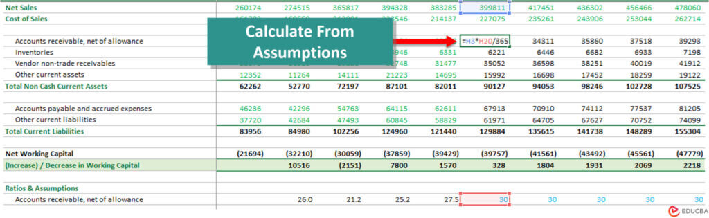
- Next, we need to calculate the Increase or (Decrease) in the working capital compared to the previous year.
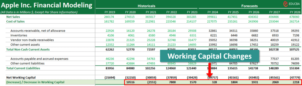
- Finally, carefully link the projected values to the Balance Sheet and Cash flows.
Step #7: Build the Depreciation Schedule
To create a complete depreciation schedule, we need to calculate several values, such as:
A. Capital Expenditure (CapEX)
B. Ending Net PPE
C. The breakup of Current PPE
D. Forecasted Breakup of PPE
E. Depreciation of Apple’s Individual Assets
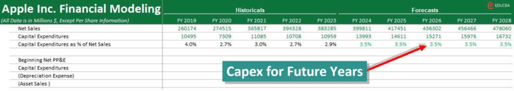
A. Steps to Calculate Capex:
- Link the “Net Sales” from the income statement to the depreciation schedule.
- Link the “Historical CapEX (2019 to 2023)” from the cash flow statement.
- Calculate CapEX as % of Net Sales for 2019 to 2023 using this formula: (CapEX / Net Sales of Previous Year) x 100.
- Based on the percentage trend for historical years, we will make percentage assumptions for future years. For instance, if the trend is 3.5%, apply this to future projections, as seen in the image below.
B. Steps to Calculate Ending Net PPE:
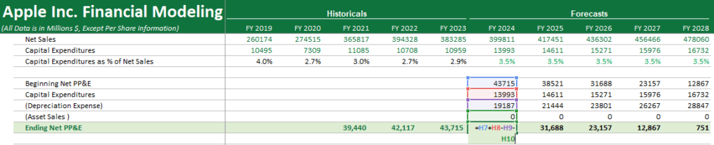
- Link the Ending Net PPE values for the historical years (2021 to 2023) from the Balance Sheet.
- Input the CapEX values (2024 to 2028) from the previous calculations.
- Calculate the Ending Net PPE for 2024 to 2028 using the below BASE equation:
- Since depreciation values for 2024 to 2028 are not yet calculated, leave them blank for now and link them later.
C. Calculate the Proportion of Assets for current PPE (2021)
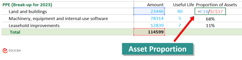
- In the “Amount” column, add the PPE numbers for FY 2023. (Refer to Apple’s 10-K Report, Page 39, for the details of PPE for FY 2023).
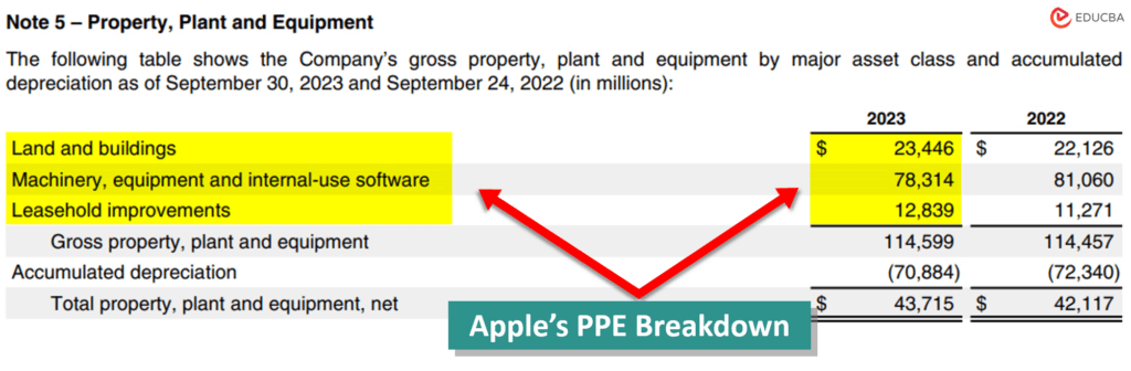
- Add the “Useful Life” of each asset in the next column. (Ensure you know the Depreciation Policy and Useful Life of Assets for the company. This information is typically disclosed in the company’s annual reports. For Apple, it’s available in their 2023 10-K Report, specifically on page 33).

- Calculate the “Proportion of Assets” using the formula:
D. Forecast Breakup of Property, Plant & Equipment (PPE)
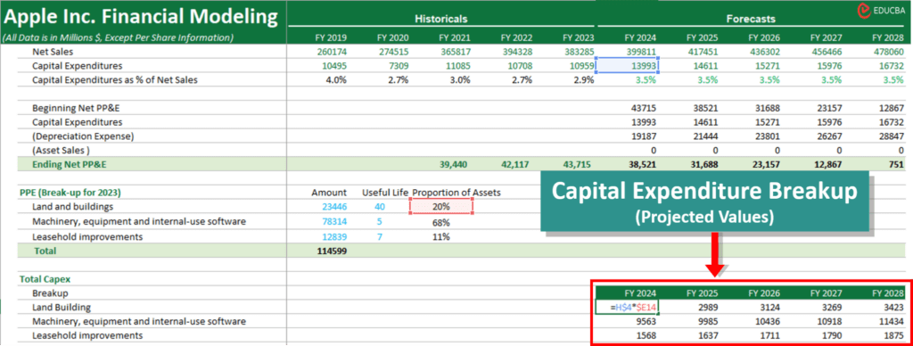
Once we estimate CapEX and the asset proportions, we can calculate the future PPE breakup.
- For example, to find the PPE breakup for Land and Buildings for FY 2024, we did the following calculation:
= CapEX value of FY 2024 × Proportion Land and Buildings
= 13993 × 20%
- Similarly, calculate for all assets and future years.
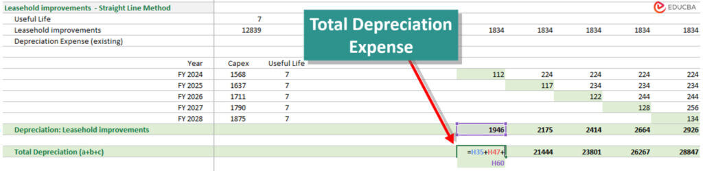
E. Calculate Depreciation of Individual Assets
1. Identify the types of assets mentioned in Apple’s annual report:
- Land and Buildings
- Machinery, equipment, and internal-use software
- Leasehold improvements.
2. For each asset type, calculate depreciation using the straight-line method, as specified in Apple’s annual report.

Depreciation Calculation Steps: Land and Buildings
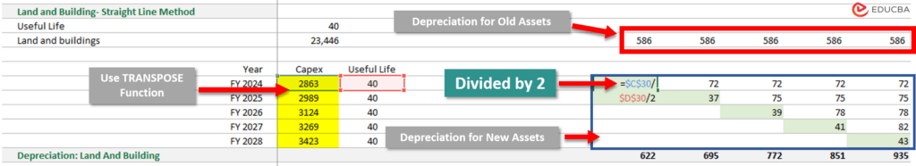
1. Transpose the CapEX values of Land and Buildings from the PPE break-up table using the TRANSPOSE function in Excel.
2. Then, we will calculate the depreciation in two parts:
- Depreciation for old assets: Calculate the depreciation for existing Land and Buildings on the Balance Sheet.
- Depreciation for new assets: Calculate the depreciation for future investments in Land and Buildings. In this case, we will divide the first forecasted year’s depreciation value by 2, assuming the assets (land and building) were bought mid-year.
3. Add depreciation for both old and new assets to arrive at total depreciation for Land and Buildings.
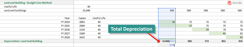
4. Repeat the above steps for all other asset types.
5. Find the total depreciation expense.
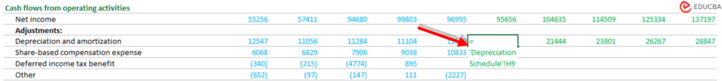
6. Link the total depreciation expense to the table to find Ending Net PPE.
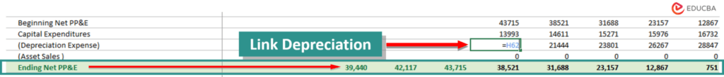
7. Link the Ending Net PPE to the Balance Sheet.
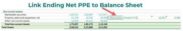
8. Link the total depreciation expense to the Cash Flow Statement.
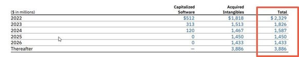
Step #8: Build the Amortization Schedule
To create a complete amortization schedule, we need to calculate these values:
- Addition to Intangibles
- Amortization of individual intangibles
We will use IBM’s amortization schedule as an example since Apple does not require a separate amortization schedule.
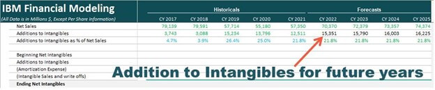
Steps to Calculate Addition to Intangibles:
- Link the “Net Sales” from the income statement and fill in the figures for the historical “Addition to Intangibles”.
- Determine Addition to Intangibles as a percentage of Net Sales for the previous years.
- If the company has provided estimated Additions to Intangibles for future years in their annual reports, that’s great! You can use those values. But if not, don’t worry; you can forecast Addition to Intangibles based on historical data, as seen in the image below.
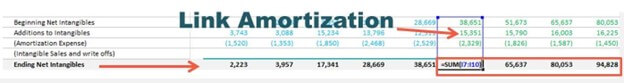
Steps to forecast the Amortization of individual intangibles:
When it comes to IBM, their intangible assets include:
- Capitalized software
- Client relationships
- Completed technology
- Patents/Trademarks
- Other** (includes acquired proprietary and nonproprietary business processes, methodologies, and systems)
Luckily, IBM has given us the forecasted amortization values in their Annual report.
We can simply link these values in the financial model and calculate the Ending Net Intangibles.
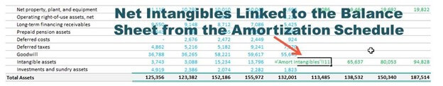
Note: Do not link this data to Apple’s financial model. We wanted to explain this process so you can use it to prepare a future financial model for another company. Having a solid understanding of financial modeling is always good
The next step is to link the Ending Net Intangibles to the Balance Sheet:
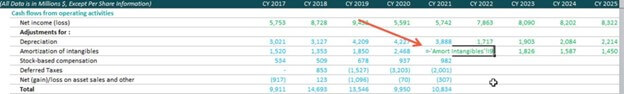
We will also link amortization to the cash flow statement:
Step #9: Build the Shareholders’ Equity Schedule
In the shareholder’s equity schedule, we aim to forecast all the equity-related items such as shareholder’s equity, retained earnings, dividends, etc.
We will start by linking historical numbers to the Shareholder’s Equity Schedule.
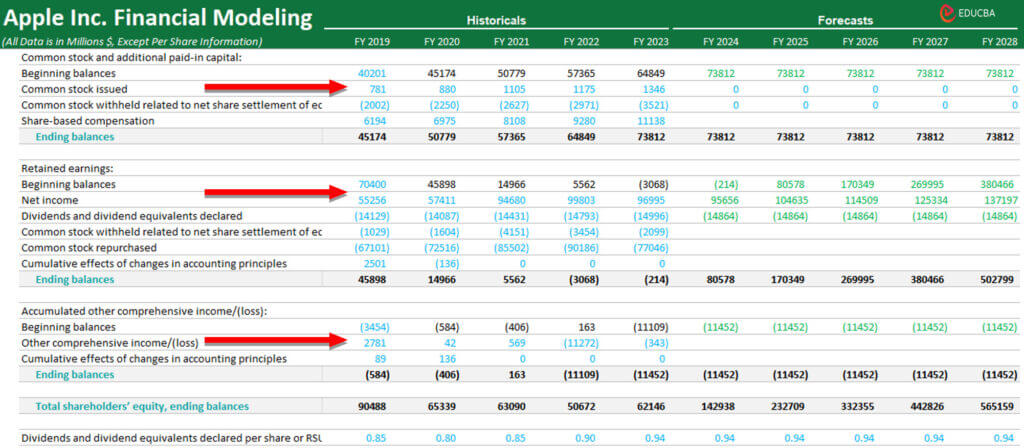
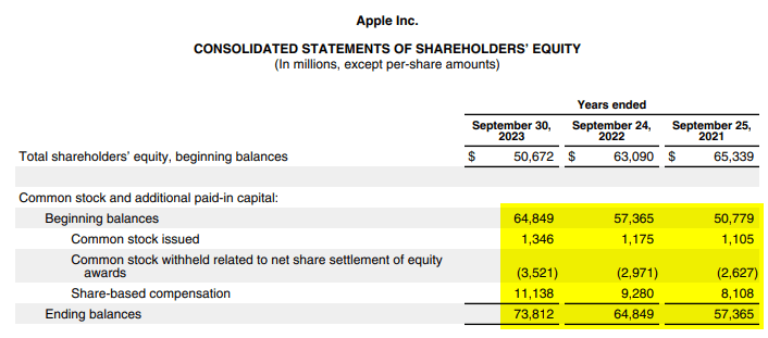
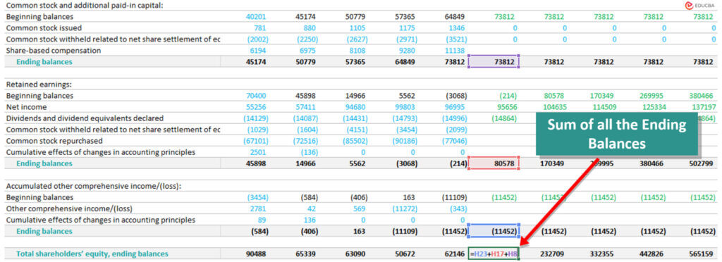
These numbers are present in Apple’s Consolidated Statements of Shareholders ‘ Equity. We can obtain details of beginning balances, common stock, retained earnings, and other comprehensive income/(loss) for Apple (Page no 31).
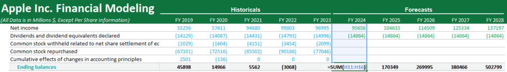
Determine the Ending Balance for Common Stock:
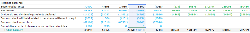
Next, determine the Ending Balance for Retained Earnings:
Determine Ending Balance for Accumulated other comprehensive income/(loss):
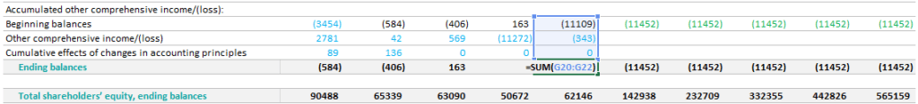
Now, finally, we will add all the Ending Balances:
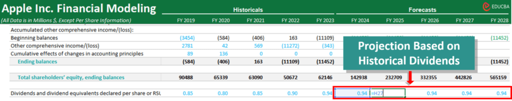
Forecast Dividends
To forecast dividends, we must first find the historical dividend payout ratio using this formula: Dividends Paid/Net Income. Using these historical payout ratio numbers, we will then assume a payout ratio to forecast dividends for future years.
1. Apple has provided us with the dividend payout ratio as “Dividends and dividend equivalents declared per share or RSU” in the annual report under “CONSOLIDATED STATEMENTS OF SHAREHOLDERS’ EQUITY” for the historicals.
2. We will directly populate those numbers in our Excel model.
3. Now, let us make assumptions based on the historical numbers. Simply link cell G27 to cell H27, hit Enter, and drag it for all future years. We assume that dividends per share will remain constant as of FY2022.
Link Ending Balances from Shareholder’s Equity Schedule to the Balance Sheet:

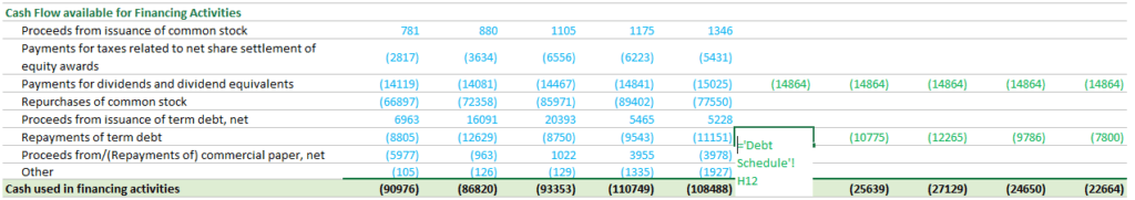
Step #10: Link and Complete the Cash Flow Statement
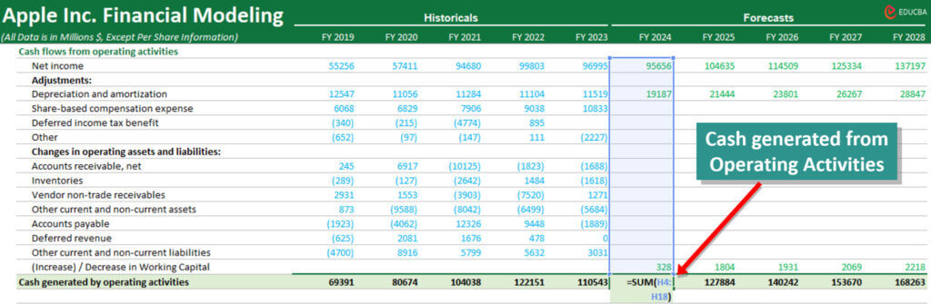
1. First, link the respective cash flows from operating activities to calculate the cash generated by operating activities.
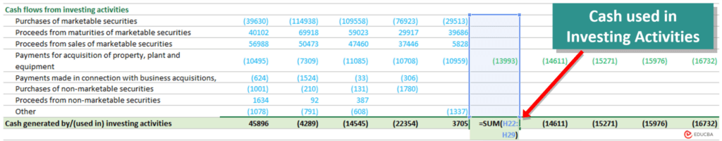
2. Link the cash used in investing activitiesand calculate the total amount below.
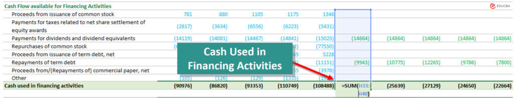
3. Then, calculate cash used in financing activities, as seen below.
Step #11: Forecast the Debt Schedule
1. Calculating Cash Available for Debt Repayment
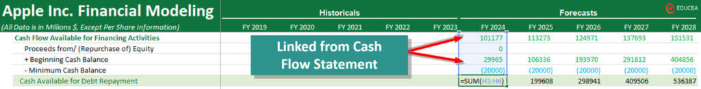
To calculate a company’s cash available for debt repayment, follow these steps.
- Link cash available for financing activities from the cash flow statement.
- Link the beginning cash balance from the cash flow statement.
- Then, assume a minimum cash balance the company needs to keep as a reserve. For our example, let’s assume a minimum cash balance of $20,000 for all forecasted years. It will depend on the company’s beginning cash balance and can vary from company to company.
2. Calculating Ending Balance of Long-term Debt
- To create a long-term debt schedule, the first step is to connect the ending balance for each historical year from the Balance Sheet.
- Once we have the ending balance for FY 2023, we will use it as the beginning balance for FY 2024, and we will link all forecasted years accordingly.
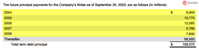
- Then, we will look for the future payments that Apple will make as provided in their annual report and populate those numbers as “Repayments”. Not all companies give this data, so that you may need additional research.
- To determine the ending balance of the long-term debt, we will simply subtract the future payments from the beginning balance.
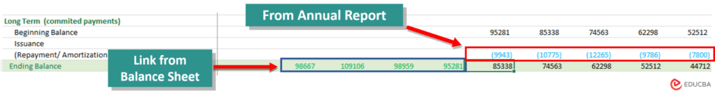
- Link Ending Balance of Long-Term Debt to Cash Flow Statement:
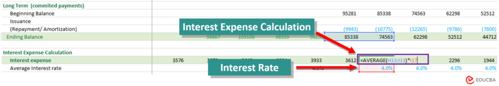
3. Interest Expense Calculation: Long-term Debt
- First, link the interest expensefrom the income statement for historical years (FY 2019 to FY 2023).
- Then, calculate the “Average interest rate” for these historical years. For example, to calculate the average interest rate for FY 2023, use this formula:
- Similarly, calculate the average interest rate for FY 2022 and the previous historical years.
- Based on historical interest rates, we will assume an interest rate of 4% for the forecasted years and start calculating the interest expense for these years.
4. Interest Income Calculation
Now, let’s link the cash and cash equivalents from the Balance Sheet to calculate interest income by taking their average. The interest rate can be considered the average saving rate that banks provide. Then, we can calculate the interest earned for each forecasted year.
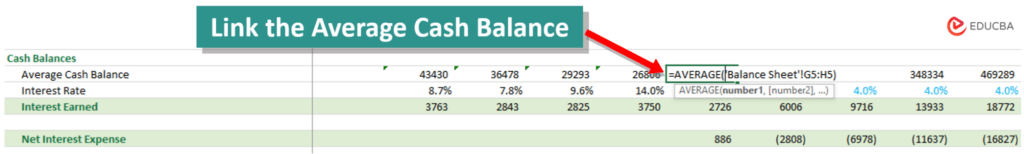
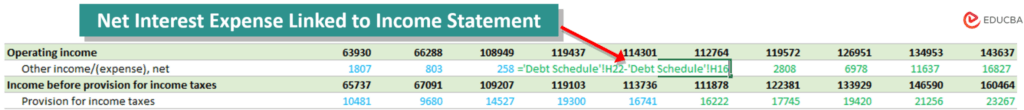
- Calculate the Net Interest Expense
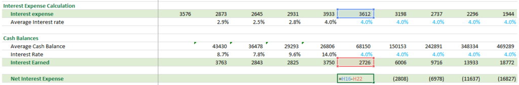
- Link the Net interest expense to the Income Statement
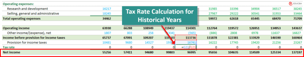
Step #12: Complete the Missing Links: Tax & Net Income
Income Tax Calculations
To calculate the “Provision for tax rate” in the Income Statement, we will calculate the tax rate for the historical years and assume a reasonable tax rate for the forecasted years.
Then, finally, we will calculate Net Income.
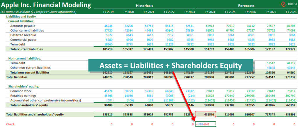
Step #13: Complete the Balance Sheet
In this step, we will complete all missing links in the balance sheet and audit it to ensure that the check is “0” everywhere. It simply means that we will ensure:
By following this process, you have successfully created a comprehensive financial model from scratch.
Financial Modeling In Excel – Infographics
Frequently Asked Questions (FAQs)
Q1. What are some important formulas for financial modeling in Excel?
Answer: Here is a list of top Excel formulas that we use in financial modeling, along with a basic example of its use:
| Excel Function | Typical Use in Financial Modeling |
| SUM | Adding a series of monthly revenues or expenses. |
| AVERAGE | Computing average monthly revenue or expense. |
| IF | Calculating revolving credit facility in debt schedule. |
| VLOOKUP and HLOOKUP | Looking up the price of a product in a price list. |
| INDEX and MATCH | Looking up the price of a product using its name and category. |
| ROUND | Rounding interest rate or tax rate to two decimal places. |
| NPV | Determine the value of a firm’s manufacturing plant, a long-term investment. |
| IRR | To determine if a particular investment is worth pursuing. |
Q2. What are some necessary financial modeling Excel shortcuts?
Answer: Knowing Excel shortcuts can simplify the process of creating a financial model in Excel. Here are a few shortcuts; however, to learn about other Excel shortcuts, check this article: Excel Keyboard Shortcuts.
- Ctrl + Enter: Enter the same data in multiple selected cells.
- Ctrl + Shift + Enter: Enter a formula as an array formula.
- Ctrl + Shift + Arrow Keys: Extend the selection to the edge of data in a particular direction.
- Ctrl + Spacebar: Select the entire column of the active cell.
- Shift + Spacebar: Select the entire row of the active cell.
Q3. Is financial modeling for startups in Excel different?
Answer: Yes, creating a financial model for startups is different as, generally, they are not public companies and don’t have their financial information readily available in annual reports. So, when it comes to predicting their future performance, we need to use methods like the top-down approach or bottom-up forecasting.
Q4. Is Excel good for financial modeling? What tool to use for financial modeling?
Answer: Excel is a good tool for building financial models. It is versatile, easy to use, and very common among finance professionals. Thus, beginners, as well as senior analysts, can use Excel to build financial models. However, if you want to use another software, you can use Oracle BI, Jirav, Cube, and more online tools.
Q5. What are the major components of financial modeling?
Answer: The company’s financial statements are the major components we use to create Excel financial modeling. A company’s financial statements include the income statement, the balance sheet, and the cash flow statements. However, use the consolidated statements from the company’s annual report, not the standalone ones.
Q6. What is the purpose of financial modeling?
Answer: The main purpose of building these models is to create a numerical representation of a company’s financial performance. It helps businesses make informed decisions about financial planning, capital allocation, and strategic investments. Another reason for building these models is to raise funds (IPO), mergers and acquisitions, etc.
Recommended Articles
We hope you were able to create an amazing financial model using this guide to financial modeling in Excel. For many other articles on financial modeling, check out the following articles.
