Updated July 1, 2023
What is Transpose in Excel?
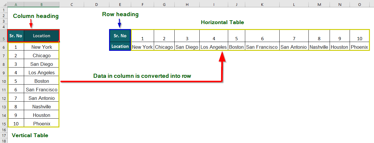
Transpose in Excel refers to a feature that allows you to flip the orientation of data in a selected range of cells, from rows to columns or from columns to rows. This means that data displayed horizontally in a row will be rearranged vertically in a column and vice versa.
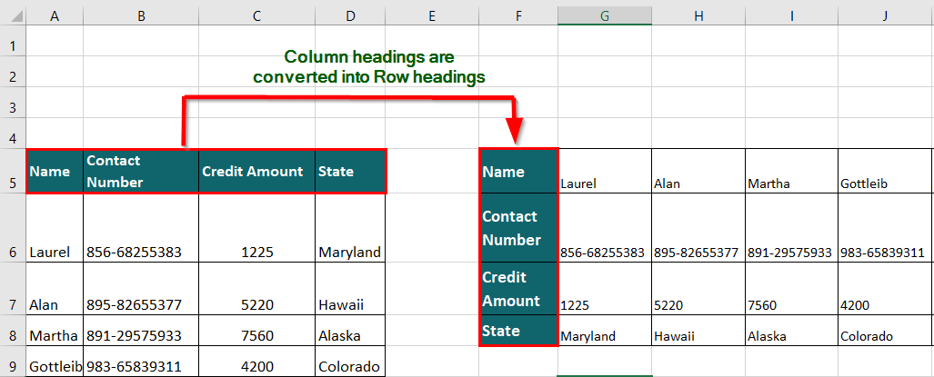
For instance, if we apply the Transpose feature in Excel to the vertical table below, it would be converted into a horizontal table. Also, the column heading is transformed into a row heading, and the data from each column is transferred into the respective rows.
This feature is especially useful when the data presentation format is inconvenient, making it difficult to analyze or visualize effectively.
Transpose in Excel Syntax
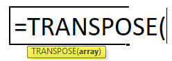
The Transpose syntax is as follows:
Key Highlights
- The Transpose function can be applied to a single cell, a range of cells, or an array.
- When a table or array is transposed, the data in the first row is moved to the first column of the new table. The second row is moved to the second column, and so on.
- The number of rows in the new table must be equal to the number of columns in the original table and the same number of columns as the old table has rows.
- The Transpose function is a built-in function in Excel, so you don’t need to write code or install add-ins.
How to use the Transpose in Excel Feature?
To transpose data in Excel, there are 2 easy methods-
1. Using the TRANSPOSE Function in Excel
To use the function Transpose in Excel worksheets, follow these steps:
- Select a range of blank cells with the number of rows equal to the number of columns of the original array and the number of columns equal to the number of rows.
- Enter the Transpose formula =TRANSPOSE(array).
- With the range still selected, Press Ctrl + Shift + Enter.
Here is an example to demonstrate these steps in detail:
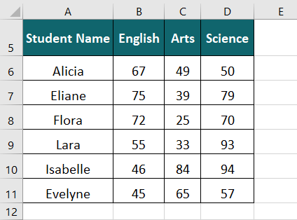
The table below shows students’ names with their marks in English, Arts, and Science. We want to transpose data in the table using the Transpose function in Excel.
Solution:
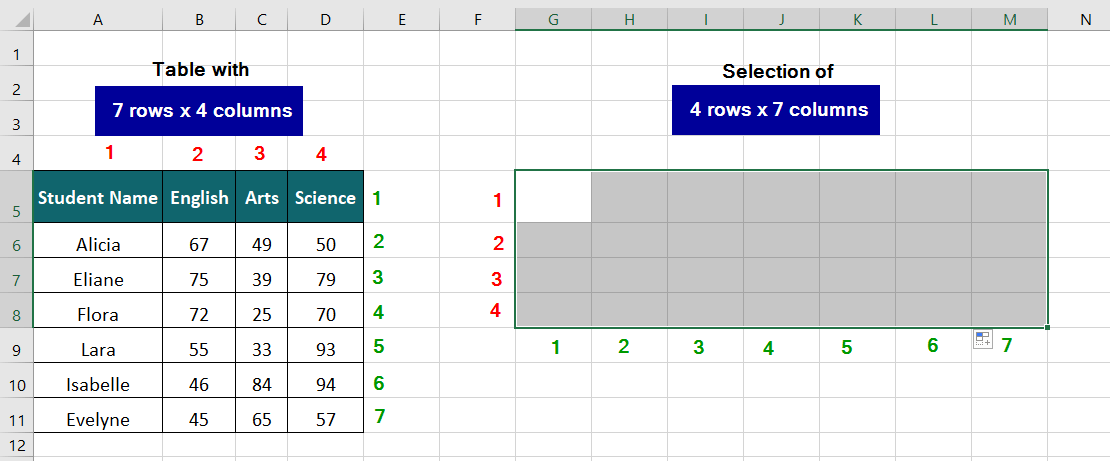
The table consists of 7 rows and 4 columns, and we want the table to be in horizontal form. To do this, we can follow the steps below:
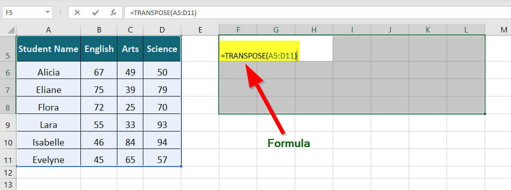
Step 1: Select the target location (cell G5) for the transposed data, which should consist of 4 rows and 7 columns, as illustrated in the image below.
Step 2: Enter the formula below into cell G5 without pressing any keys.
Where,
A5:D11 is the (source) array we want to transpose.
Step 3: Press the keys CTRL + SHIFT + ENTER.
The result of pressing CTRL + SHIFT + ENTER is inserting a set of braces around the formula, which can be seen in the following image.
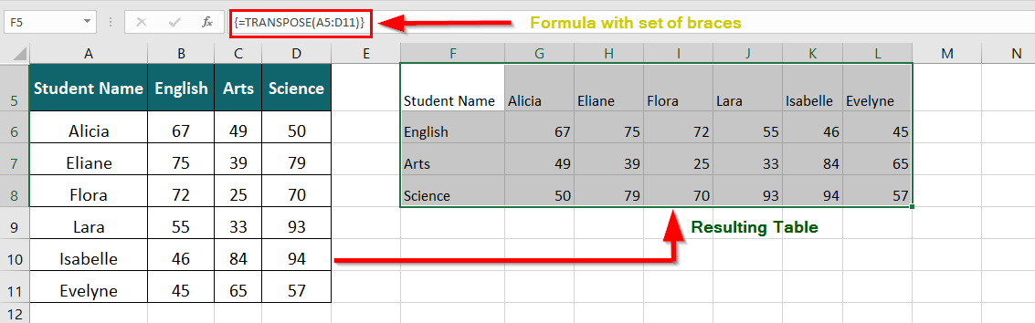
The Transpose in Excel function converts the vertical table into a horizontal table, i.e., the column headings are switched as row headings, and the column values are transferred to the rows.
2. Using Copy-Paste Feature
To use the Copy-Paste feature to Transpose in Excel, follow these steps:
- Select the range of cells you want to transpose.
- Right-click on the selection and choose “Copy” or use the “Ctrl + C” shortcut.
- Right-click on a blank cell where you want to paste the transposed data.
- Choose “Paste Special” from the context menu.
- In the Paste Special dialog box, check the Transpose” option.
- Click “OK” to transpose the data.
Below is an example to demonstrate the above steps in detail:
Example #1
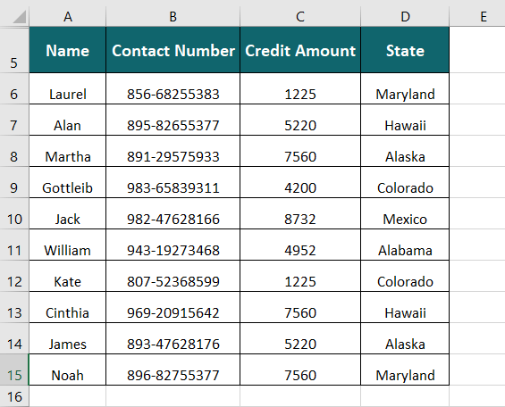
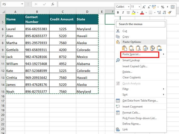
The vertical table below shows a list of beneficiaries with their contact number, credit amount, and the states they belong to. We will use the Copy-Paste feature of Excel to transpose the columns and rows of the data.
Solution:
Step 1: Select the above table to transpose.
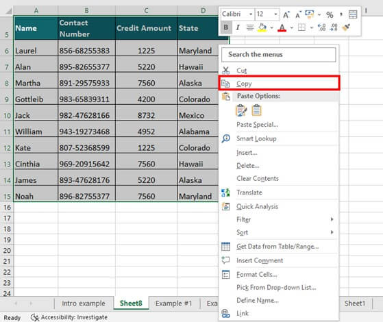
Step 2: Right-click the selection and choose Copy. Alternatively, use the shortcut Ctrl + C.
Step 3: Right-click on a blank cell (F5) where you want to paste the transposed data.
Step 4: Choose Paste Special from the context menu.
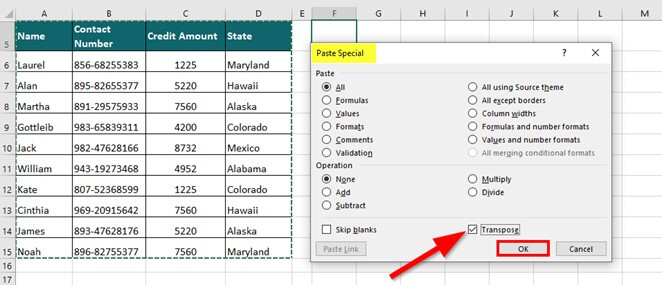
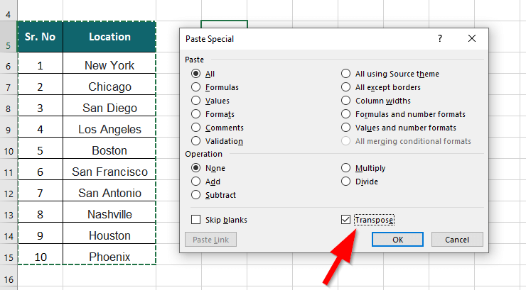
A Paste Special dialog box appears.
Step 5: Click the Transpose checkbox and click OK.
The Vertical Table is converted into a Horizontal table, as shown below
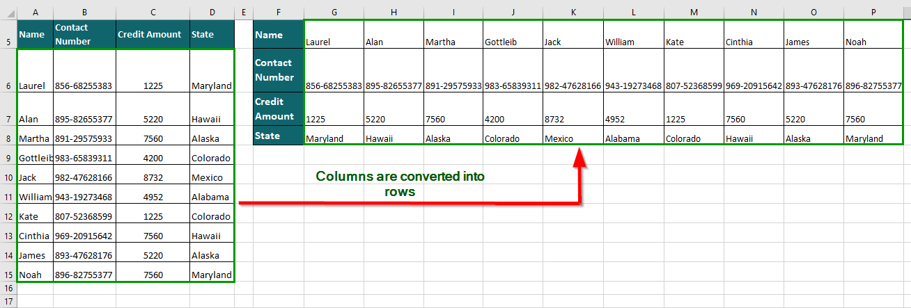
The data in the column is shifted to rows
The column headings are transferred into row headings.
Example #2
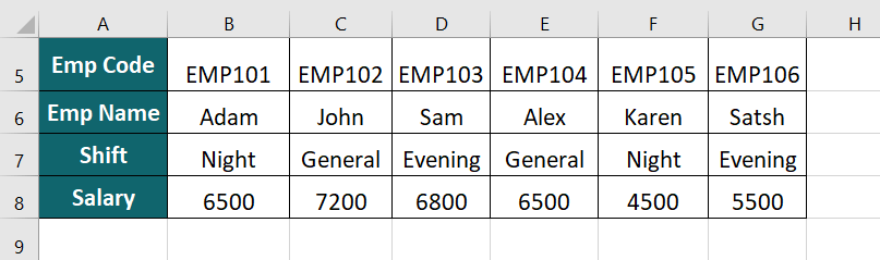
The horizontal table below shows Employee Code, Employee name, Shift, and Salary. We want to transpose the table into a Vertical form using the Copy-Paste feature in Excel.
Solution:
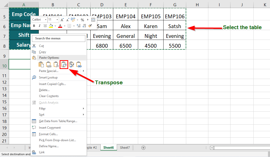
Step 1: Select the table and right-click at the location (cell A10) where you want the new table.
A list of options will appear,
Step 2: In the Paste Options section, click on the Transpose icon as shown below
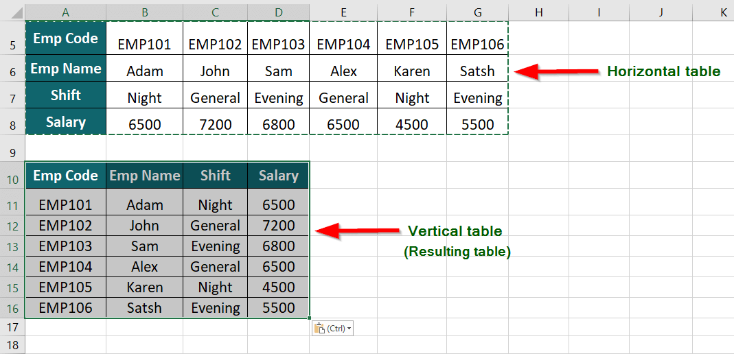
The Horizontal table is converted into a vertical table, i.e., row headings become column headings and values in the rows are shifted to the columns.
We cannot use the Copy-paste transpose feature if we want to change the source data. The changes will not reflect in the new table (array).
Things to Remember
When using the Transpose function in Excel, several things must be remembered to ensure that the data transposes accurately and without errors. Here are some important things to remember:
- The Transpose function must be used on a selection of the same size and shape as the original data. For example, if you have a table with three rows and four columns, the selection that one uses with the Transpose function must be four rows and three columns.
- The data to be transposed must not contain any merged cells, as this can cause the function to fail or produce unexpected results.
- The Transpose function can only be used on data not formatted as a table. To transpose a table, you must first convert it to a range.
- It is essential to select the destination range carefully. If the destination range contains any existing data, it will be overwritten with the transposed data.
Finally, it’s important to remember that the Transpose function only transposes data; it does not sort or filter it. If you need to sort or filter the transposed data, you will need to use other Excel functions.
Final Thoughts
The Transpose function in Excel is an essential tool for anyone who works with large datasets or wants to reformat data quickly and efficiently. By mastering the Transpose function, you can transform complex data sets into a more manageable and understandable format, making it easier to analyze, visualize, and make informed decisions based on the data.
Frequently Asked Questions (FAQs)
Q1. Where is Transpose in Excel?
Answer: The Transpose feature in Excel is available in the “Paste Special” dialog box.
Here are the steps to access the Transpose feature:
- Select the cells that you want to transpose.
- Right-click on the selection and choose “Copy” or use the “Ctrl + C” shortcut.
- Right-click on the cell where you want to paste the transposed data.
- Choose “Paste Special” in the context menu or use the “Ctrl + Alt + V” shortcut.
- In the Paste Special dialog box, check the “Transpose” option.
- Click “OK” to transpose the data.
Q2. What is the importance of transposing data?
Answer: Transposing data in Excel can be important for several reasons:
- Changing the orientation: Transposing can help change the orientation of data from rows to columns or vice versa, making it easier to read or work with the data differently.
- Analyzing data: Transposing can be useful when you want to analyze data in a specific way, such as comparing different data sets or performing calculations across multiple rows or columns.
- Preparing data for charts or graphs: Certain types of charts or graphs require data to be in a specific orientation, and transposing can help you prepare the data accordingly.
- Importing or exporting data: When importing or exporting data between different systems or applications, you may need to transpose the data to match the expected format or structure.
Q3. What does transposing data mean?
Answer: Transposing an array or a dataset means swapping columns and rows so that the columns become rows and rows become columns.
For example, if you have a table of sales data where each row represents a different product and each column represents a different month, transposing the data would change the orientation so that each row represents a different month and each column represents a different product. This can be useful for certain calculations or for visualizing the data differently.
Q4. Is there a transpose formula in Excel?
Answer: Yes. The Transpose formula is,
=TRANSPOSE(array)
For example, if you want to transpose the range A1:E4, you would enter the following formula in a cell where you want the transposed data to start:
=TRANSPOSE(A1:E4)
Once you have entered the formula, press Ctrl + Shift + Enter and the transposed data will be displayed.
Recommended Articles
This has been a guide to the TRANSPOSE Function. Here we discuss the TRANSPOSE Formula, how to use the TRANSPOSE Function, practical examples, and downloadable Excel templates. You can also go through our other suggested articles –
