Updated June 8, 2023
AVERAGE in Excel
The average function calculates the average of the selected numbers or digits in the same logic as we used in mathematics. The average function calculates the sum of selected numbers and then divides the outcome from summation by the total numbers selected in the range. Thus, choosing the Average function overdoing the process to calculate the average is 2 fewer steps. Therefore, sometimes we have seen average to be called MEAN, but it will be available as AVERAGE in Excel.
The AVERAGE function is categorized under Statistical functions. It is used as a worksheet & VBA function in Excel.
- According to the mathematical definition, Arithmetic mean, or Average is calculated by adding numbers together, then dividing the total by how many numbers are being averaged.
- Its most commonly used function is in the financial & statistical domain, where it will be helpful to analyze yearly average sales & revenue for a company.
- Thus, it is simple & easy to use Excel function with few arguments
Definition
AVERAGE: Calculate the arithmetic mean or average of a given set of arguments
AVERAGE Formula in Excel:
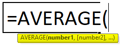
Below is the AVERAGE Formula:
The Formula or Syntax for an Average function is:
Where
Number 1: Numeric values for which we want to find the average; the first argument is compulsory & it is required. Subsequent arguments are optional, i.e. (from Number 2 onwards)
Arguments can be given as numbers or cell references, or ranges
Up to 255 numbers can be added
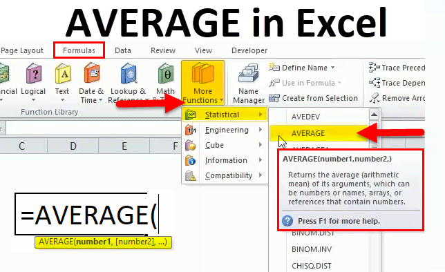
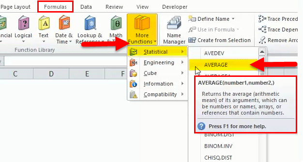
How to Use the AVERAGE Function in Excel?
The AVERAGE Function is very simple to use. Let us now see how to use the AVERAGE function in Excel with the help of some examples.
Example #1
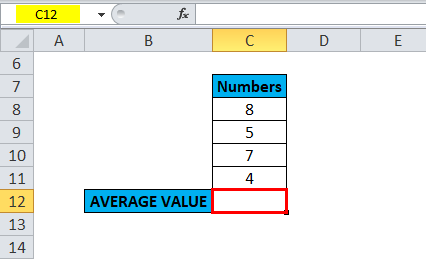
AVERAGE Calculation for a set of Numbers
With the help of the Average function, I need to find out the average of given numbers in the cell.
Let’s apply the Average function in cell “C12”. Select the cell “C12,” where an Average function needs to be applied.
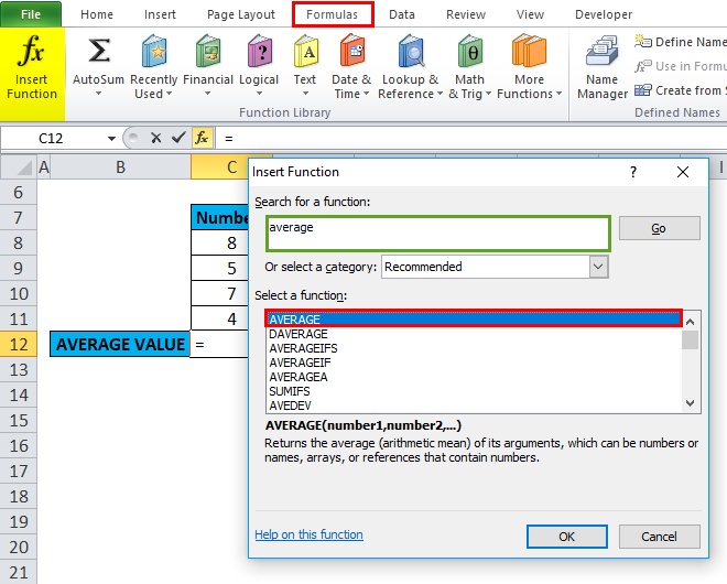
Click the insert function button (fx) under the formula toolbar; a dialog box will appear, type the keyword “AVERAGE” in the search for a function box, and an AVERAGE function will appear in Select a function box. Double-click on an AVERAGE function.
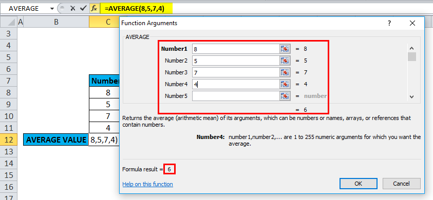
A dialog box appears where arguments for the average function need to be filled or entered, i.e., =Average (Number1, [Number 2]…). You can enter the numbers directly into the number arguments in cells C8 TO C11.
Click ok after entering all the numbers.
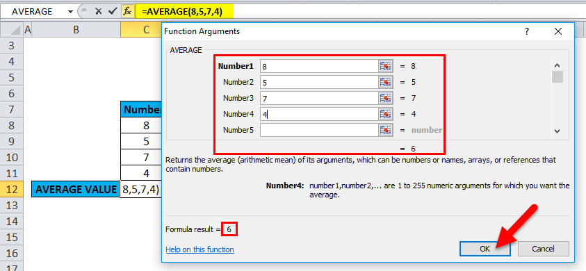
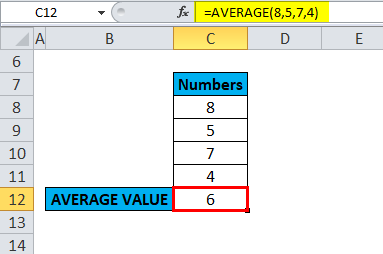
i.e., =AVERAGE(8,5,7,4) returns 6 as a result.
Example #2
To Calculate AVERAGE for Rows & Columns of data
A) Average function for column range
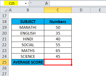
In the below-mentioned example, the Table contains subject-wise marks or scores of a student in column C (C19 TO C24 is the column range)
With the help of the Average function, I need to find out the average score of a student in that column range (C19 TO C24 is the column range). Let’s apply the Average function in cell “C25”. Select the cell “C25,” where an Average function needs to be applied.
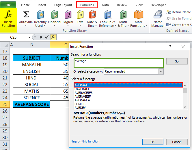
Click the insert function button (fx) under the formula toolbar; a dialog box will appear, type the keyword “AVERAGE” in the search for a function box, and an AVERAGE function will appear in the select a function box. Double-click on an AVERAGE function
A dialog box appears where arguments for the AVERAGE function need to be filled or entered, i.e., =Average (Number1, [Number 2]…). Here, we need to enter the column range in the Number1 argument, click inside cell C19, and you’ll see the cell selected, then Select the cells till C24. So that column range will get selected, i.e., C19:C24. Click ok after entering the column range.
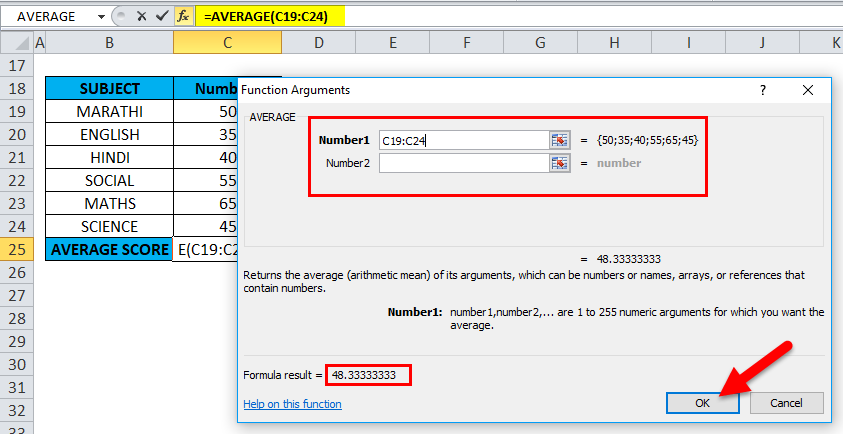
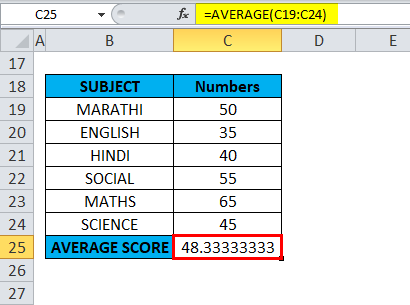
i.e., =AVERAGE(C19:C24) returns 48.33333333 as a result. The average subject score is 48.33333333
B) Average function for row range
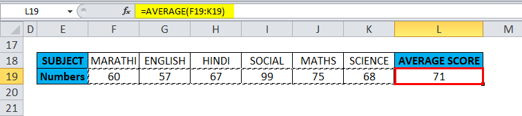
In the below-mentioned example, the Table contains subject-wise marks or scores of a student in row number 19, i.e., score or number row (F19 TO K19 is the row range)
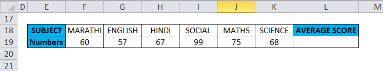
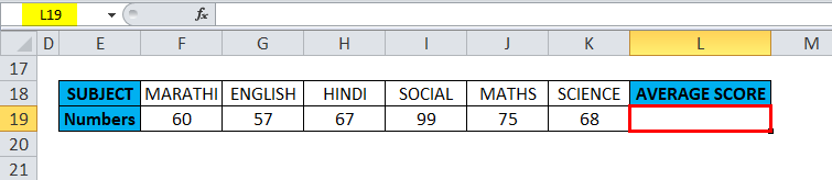
With the help of the Average function, I need to find out the average score of a student in that row range (F19 TO K19). Let’s apply the Average function in cell “L19”. First, select the cell “L19,” where an Average function needs to be applied.
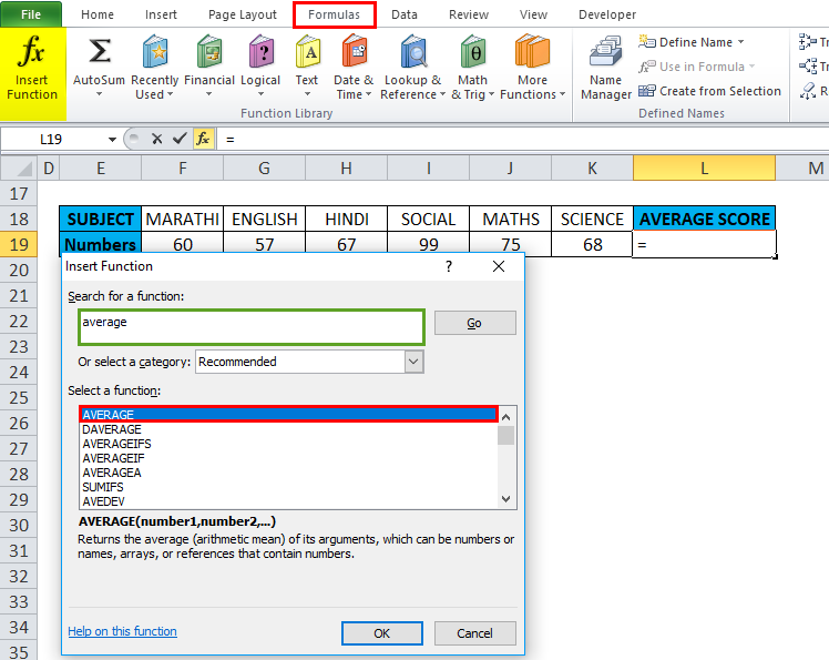
Click the insert function button (fx) under the formula toolbar; a dialog box will appear, type the keyword “AVERAGE” in the search for a function box, and an AVERAGE function will appear in Select a function box. Double-click on an AVERAGE function.
A dialog box appears where arguments for the AVERAGE function need to be filled or entered, i.e., =Average (Number1, [Number 2]…).
Here, we need to enter the Number1 argument; click inside cell F19, and you’ll see the cell selected and then Select the cells until K19. So that row range will get selected, i.e., F19:K19. Click ok after entering the row range.
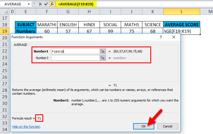
i.e., =AVERAGE(F19:K19) returns 71 as a result. The average subject score is 71
Example #3
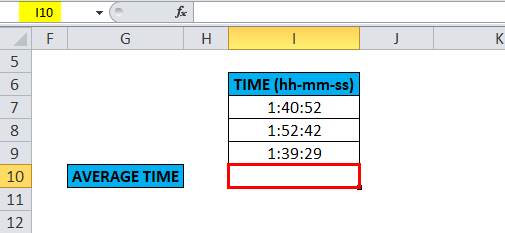
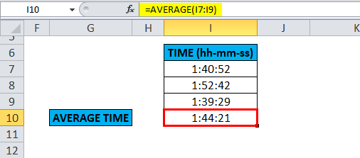
To Calculate the AVERAGE Time
The average function helps calculate the average time that includes hours, minutes, and seconds for a marathon race.
The table below contains the time data of the top three racers, i.e., the Time they took to finish the race. (in hours, minutes, and seconds format)
With the help of the average function, I need to find the average time. Let’s apply the Average function in cell “I10”. Select the cell “I10”. where the Average function needs to be applied.
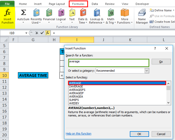
Click the insert function button (fx) under the formula toolbar; a dialog box will appear, type the keyword “AVERAGE” in the search for a function box, and an AVERAGE function will appear in Select a function box. Double-click on the AVERAGE function.
A dialog box appears where arguments for the AVERAGE function need to be filled or entered, i.e., =Average (Number1, [Number 2]…).
Therefore, we need to enter the Number1 argument; click inside cell I7, and you’ll see the cell selected, then Select the cells till I9. So that column range will get selected, i.e., I7:I9. Click ok after entering the column range.
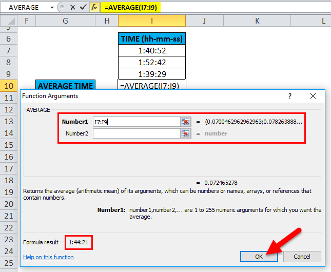
i.e. =AVERAGE(I7:I9) returns 1:44:21 as the result. The average time value is 1:44:21
Things to Remember
- Cells containing Boolean operators, text strings, TRUE, FALSE, and empty or blank cells will be ignored (Note: it will not ignore the cells with the value zero)
- If any supplied arguments are entered directly and cannot be interpreted as numeric values, it gives #VALUE! Error G. = AVERAGE (“Two”, “Five”, “Six”)
- If any of the supplied argument is arguments are non-numeric, it gives #DIV/0! Error
- The AVERAGE function differs from the AVERAGE A function, where an AVERAGE function is used to find an average of cells with any data, i.e., text values, numbers, and Boolean.
- The AVERAGE function is not restricted to finding the average of a table range or row range or column range, or non-adjacent cells. Instead, you can specify individual cells in number arguments to get the desired results.
Recommended Articles
Thus, this has been a guide to the Excel AVERAGE function. Therefore, we discuss the AVERAGE Formula and how to use an AVERAGE function in Excel, with practical examples and a downloadable Excel template. You can also go through our other suggested articles –
