MATCH in Excel
The MATCH function is a powerful tool in Excel that helps users search for a specific value within a range of cells and return its relative position. It’s a useful function for those who work with large datasets or need to locate specific values quickly.
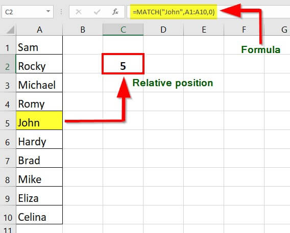
For instance, consider a situation where you have a long list of names, and you need to find the position of a particular name (John) within that list. You can use the MATCH function to search for the name and get its position (5).
The utility of the MATCH function extends beyond simple searches within a range. For instance, one can use it in conjunction with other functions like INDEX and OFFSET to perform more complex operations.
Key Highlights
- The MATCH function in Excel can perform both exact and approximate matches.
- It can perform partial matches using wildcard operators such as * and ?.
- The MATCH function returns a #N/A error if it does not find a match in the given array.
- By using the MATCH and INDEX functions together, one can avoid using the VLOOKUP function to find a value at a matched position.
- The Match type is an optional argument in the MATCH function, and if not specified, it defaults to 1.
Syntax of MATCH Function in Excel
The syntax of the MATCH function is as follows:
1. Lookup_value (required): Indicates the value whose position we want to find in the selected range. A lookup value can be text, number, logical value, or cell reference.
2. Lookup_array (required): The cell range that contains the lookup value. Lookup array can be a row or a column.
3. Match_Type (optional): An optional argument with values 1, 0, and -1. The match_type argument, set to 0, returns an exact match, while the other two values allow for an approximate match.
a) Match_Type “1”: If the match type value is set as 1, Excel provides a value less than or equal to the lookup value.
b) Match_Type “0”: If the match type value is set as 0, Excel provides the first value that is equal to the lookup value.
c) Match_Type “-1”: If the match type value is set as 0, Excel provides the smallest value that is greater than or equal to the lookup value.
Types of MATCH Function in Excel
Here are the different types of MATCH functions in Excel:
#1 Exact MATCH
The MATCH function performs an exact match when the match type is set to zero. In the below-given example, the formula in E3 is:
Here, the MATCH Function returns the Exact match as 4.
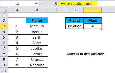
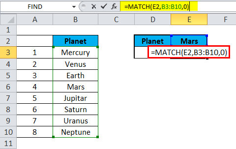
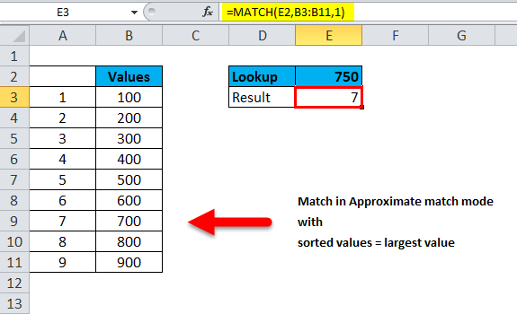
#2 Approximate MATCH
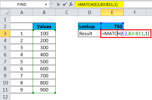
MATCH will perform an approximate match on values sorted A-Z when the match type is set to 1, finding the largest value less than or equal to the lookup value. The MATCH in Excel returns an approximate match as 7. In the below-given example, the formula in E3 is:
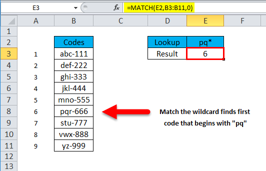
#3 Wildcard MATCH
The MATCH function can perform a match using wildcards when the match type is zero.
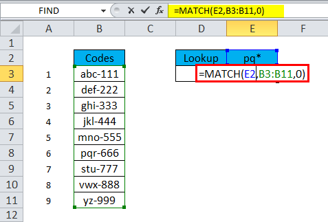
The MATCH function returns the result of wildcards as “pq”. In the below-given example, the formula in E3 is:
Points to Note
- A MATCH Function is not case-sensitive.
- MATCH returns the #N/A error if there is no match is found.
- The argument lookup_array must be in descending order: True, False, Z-A,…9,8,7,6,5,4,3,…, and so on. However, if match_type is set to 1 or omitted, the lookup_array must be sorted in ascending order.
- The wildcard characters like an asterisk () and question mark (?) can be used in the lookup_value argument if match_type is set to 0 and lookup_value is in text format, regardless of whether the lookup_value contains these characters. The asterisk () matches any sequence of characters, while the question mark (?) matches any single character.
How to Use the MATCH Function in Excel?
Example #1 Finding The Exact Match
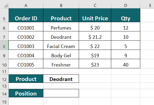
The table below lists ordered products with their order ID, unit price, and sales quantity. We want to find the position of “Deodorant” in the table using the MATCH function in Excel.
Solution:
Step 1: Select the cell where you want to display the product “Deodorant” position. In this case, let’s assume it is cell B12.
Step 2: Type the MATCH function in the formula bar: =MATCH(B12, B6:B10,0)
- The first argument in the formula is the lookup value, which is “Deodorant“, i.e., cell B12.
- The second argument of the MATCH function is the lookup array, which is the range B6:B10. This range contains the products listed in the table.
- The third argument of the MATCH function is the match type, which is 0. This means we want to find an exact match of the lookup value in the array.
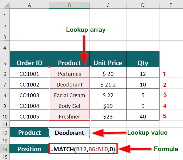
Step 3: Press Enter to get the result, as shown below.
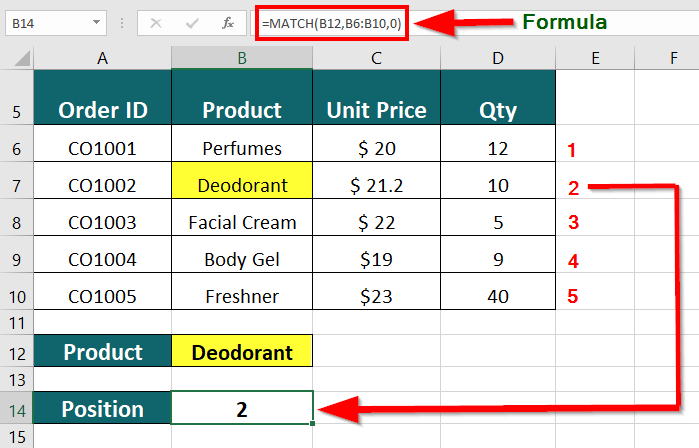
The formula returns the position of “Deodorant” in the table, which is 2. This means that “Deodorant” is the second product listed in the table.
Explanation of the Formula:
When you press the Enter key, Excel searches through the cells in the lookup array “B6:B10” to find an exact match for the lookup value “Deodorant”. After finding the match, it returns the position of the first cell containing the lookup value. In this scenario, the formula returns the value “2“, indicating that the first cell containing “Deodorant” is the second cell in the range B6:B10.
Example #2 Finding Partial MATCH using Wildcard Character
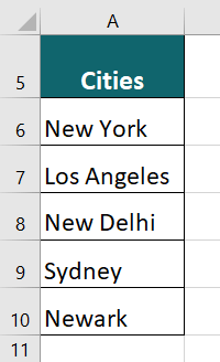
Let’s say we have a list of cities in Column A, and we want to find the position of the city that starts with “New” in the list.
Here’s how we can do it:
Step 1: Open a new Excel spreadsheet and enter the list of cities in Column A.
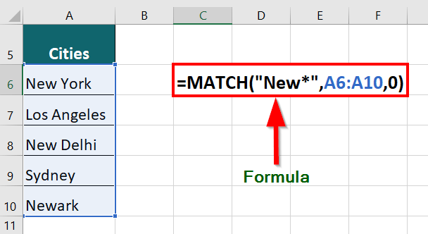
Step 2: Enter the formula =MATCH(“New*”, A6:A10,0) in an empty cell.
Explanation of the Formula:
- “New*”: This is the search criteria. The asterisk () is a wildcard character representing any number of characters. So, “New” will match any city name that starts with “New”.
- A6:A10: This is the range of cells in which we want to search for our city name.
- 0: This is the match_type argument. Here, we’re using an exact match, so we specify 0.
Step 3: Press the “Enter” key to display the result in the cell where you entered the formula.
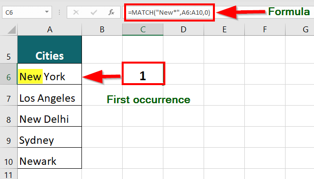
The result is “1,” which is the first city’s position starting with “New”. In this case, “New York” is the first city that starts with “New” in the list.
Example #3 Using INDEX and MATCH Function Together
The table below shows a list of students with marks in the subjects – Language, Maths, History, and Physics. Using the INDEX and MATCH functions together, we want to find Alex’s marks in History.
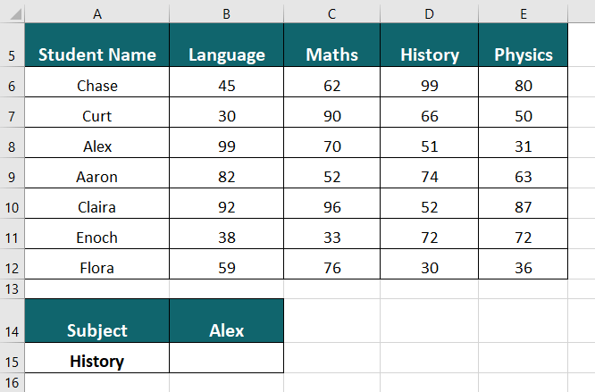
Solution:
Step 1: Select the cell where you want to display the result. In this case, it is cell B15.
Step 2: Enter the formula in the cell:
- A5:E12: This is the range of cells containing the student data table.
- B14: This is the value we want to find in the first column of the table, which is the name of the student whose marks we want to find (in this case, “Alex”).
- A5:A12: The range of cells containing the students’ names in the table’s first column.
- 0: This argument specifies that we want an exact match.
- A15: This is the value we’re looking for in row 5, which is the subject “History”.
- A5:E5: This is the cell range containing the subject names.
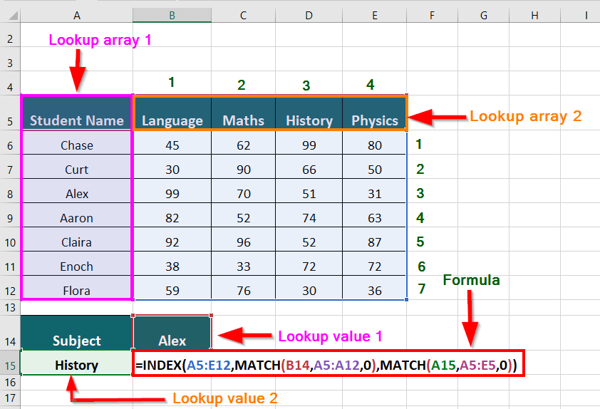
Step 3: Press Enter key to get the below result.
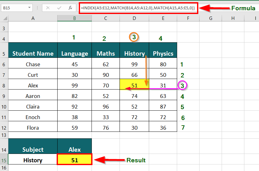
The INDEX and MATCH functions of Excel work together to provide the result of 51, which denote History marks of Alex.
Explanation of the Formula:
- The first MATCH function in the formula =INDEX(A5:E12, MATCH(B14, A5:A12,0), MATCH(A15, A5:E5,0)) searches for the student name “Alex” in the range A5:A12 and returns the relative position of that name within the range. In this case, “Alex” is in the third row of the range, so the first MATCH function returns the value 3. The third argument of the MATCH function is 0, which specifies that we want an exact match.
- The second MATCH function in the formula searches for the subject “History” in the range A5:E5 and returns the relative position of that subject within the range. In this case, “History” is in the third column of the content, so the second MATCH function returns the value 3. Again, the third argument of the MATCH function is 0, which specifies that we want an exact match.
- The INDEX function then uses these two values (3 and 3) to return the corresponding value in the table, which is Alex’s marks in History (51).
Example #4 When a Cell contains One of Many Things
Generic formula: {=INDEX(results,MATCH(TRUE,ISNUMBER(SEARCH(things,A1)),0))}
Explanation: The INDEX / MATCH function formed on the SEARCH function can be used to check a cell for one of many things and give back a custom result for the first match found.
In the example shown below, the formula in cell C5 is:
{=INDEX(results,MATCH(TRUE,ISNUMBER(SEARCH(things,B5)),0))}
Since the above is an array formula, it should be entered using the Control + Shift + Enter keys.
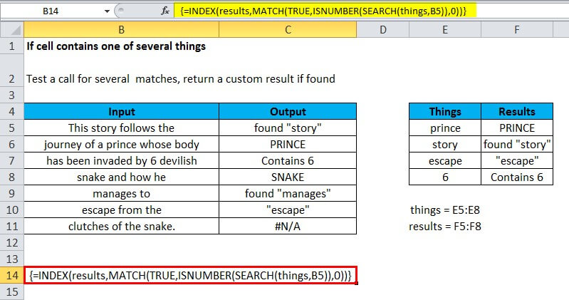
Explanation of the Formula:
- This formula uses two named ranges: E5:E8 is named “things”, and F5:F8 is named “results”.
- Ensure using the name ranges with the same names (depending on the data). If one doesn’t want to use named ranges, use absolute references instead.
- The main part of this formula is the below snippet:
ISNUMBER(SEARCH(things, B5)
- This is based on another formula that checks a cell for a single substring. If the cell has the substring, the formula gives TRUE; if not, the formula gives FALSE.
Example #5 Lookup using the Lowest Value
Generic formula =INDEX(range,MATCH(MIN(vals),vials,0))
Explanation: To look up information associated with the lowest value in a table, one can use a formula depending on MATCH, INDEX, and MIN functions.
In the below example, a formula is used to find the contractor’s name with the lowest bid. The formula in F6 is:
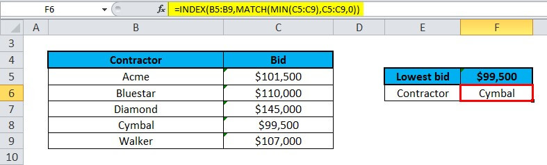
Explanation of the Formula:
- Working from the inside out, the MIN function is generally used to find the lowest bid in the range C5:C9:
- The result, 99500, is fed into the MATCH function as the lookup value:
- MATCH then gives back the position of this value in the range 4, which goes into INDEX as the row number and B5:B9 as the array:
=INDEX(B5:B9, 4) // returns Cymbal
- The INDEX function then gives back the value at that position: Cymbal.
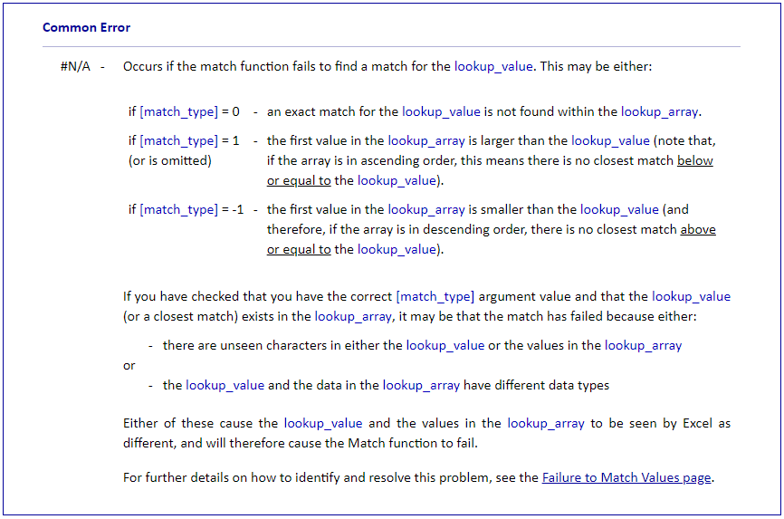
Match Function Errors
If you get an error from the Match function, this is likely to be the #N/A error:
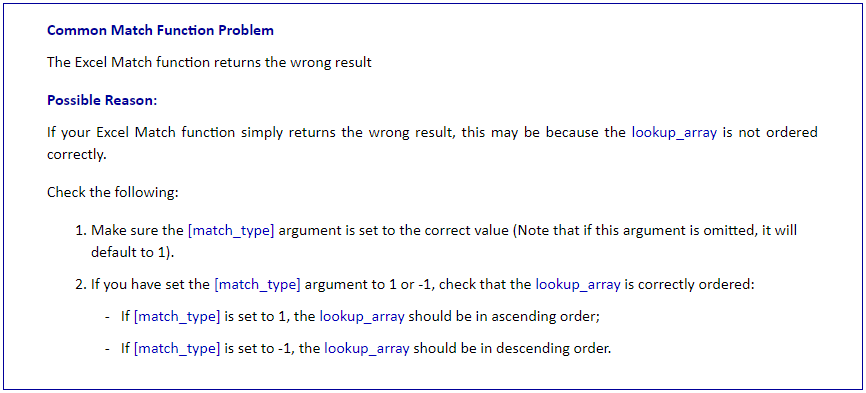
Also, some users experience the following common problem with the Match Function:
Things to Remember
- MATCH types: One can use three match types with the MATCH function: 0, 1, and -1. The default match type is 0, which finds an exact match. Match type 1 finds the largest value less than or equal to the lookup_value, while match type -1 finds the smallest value greater than or equal to the lookup_value.
- Array size: The lookup_array argument must be a one-dimensional array or a reference to a one-dimensional range of cells. If the lookup_array is not one-dimensional, the MATCH function will return a #N/A error.
- Sorted order: If the values in the lookup_array are not sorted in ascending order, the MATCH function in Excel may return an incorrect result. In such cases, use the match_type argument to specify the appropriate match type.
- Exact MATCH: If the MATCH function does not find the lookup_value in the lookup_array, it will return a #N/A error. You can use the IFERROR function to handle this error and return a more meaningful result.
- Relative or absolute cell reference: The MATCH function is compatible with both relative and absolute cell references. When copying the formula to other cells, the function will adjust the cell references accordingly.
Frequently Asked Questions (FAQs)
Q1. What is an example of a MATCH function in Excel?
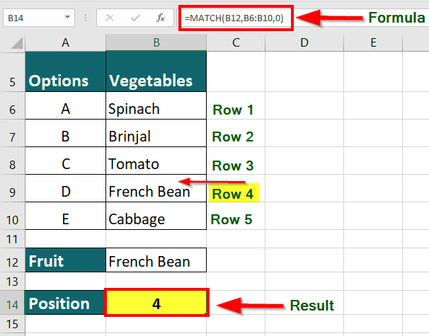
Answer: The MATCH function searches for a given value in a data set and provides the position of that value in the range. For instance, suppose you have a data set that includes items like Spinach, Brinjal, Tomato, French Bean, and Cabbage in the range B6:B10. If you want to find the position of the value “French Bean” in the range, you can use the MATCH function.
The formula =MATCH(B12, B6:B10,0) returns the “French Bean” position in the range B6:B10 as the number 4.
Q2. What is the benefit of including the MATCH function within an INDEX function?
Answer: Including the MATCH function within an INDEX function allows you to retrieve data dynamically based on specific search criteria.
Suppose you have a list of fruits and their prices in a table. You want to retrieve the price of a specific fruit, say “Apple”, from the table. One way to do this is to search the table for the row containing “Apple manually” and then look for the price in the corresponding column. However, if you have a large dataset with many rows and columns, this can be a time-consuming and error-prone process. Instead, you can use the MATCH function to find the “Apple” row number in the table and then use the INDEX function to retrieve the price from the corresponding column. The formula would look like this:
The MATCH function searches for “Apple” in the table’s first column (A2:A6) and returns the row number where it is found. The INDEX function then retrieves the value from the table’s third column (price column) at the intersection of the row and column numbers that the MATCH function returns.
Q3. Can the MATCH function have multiple criteria?
Answer: It is possible to use the MATCH function with multiple criteria by combining it with other functions such as INDEX, SUMPRODUCT, and COUNTIFS. For instance, consider this formula:
This formula uses MATCH with multiple criteria to find the position of the first employee in the “Sales” department who earns more than $20,000 per year. Then, it adds the count of cells that satisfy only the second condition using the COUNTIFS function.
Q4. What is the difference between MATCH and VLOOKUP in Excel?
Answer: The MATCH function helps us find the location of a particular value in a column or row, while the VLOOKUP function helps us retrieve information associated with that value.
For instance, if we want to find the price of oranges in the following table, we will have to use the MATCH function in conjunction with the INDEX function to find the price. Alternatively, the VLOOKUP function can directly provide the price of oranges at $0.75.
|
Product |
Price |
| Apples | $1.00 |
| Oranges | $0.75 |
| Bananas | $0.50 |
The formula for using MATCH and INDEX functions together is =INDEX(B: B, MATCH(“Oranges”, A: A, 0)). Using MATCH, this formula finds the position of “Oranges” in column A, which returns the value 2. Then, INDEX retrieves the value in column B’s corresponding row, i.e., $0.75.
- The VLOOKUP function formula is =VLOOKUP(“Oranges”, A: B, 2, 0). This formula looks for “Oranges” in the first column of the range A: B and returns the corresponding value from the second column (i.e., the price column), resulting in $0.75.
Recommended Articles
The above article is our guide to using the MATCH function in Excel. Here are some further examples of expanding understanding:
