Updated July 19, 2023
What is the INDEX Function in Excel?
The INDEX function in Excel provides the value of a cell within a selected range against a given row and column. For example, the formula = INDEX(“Employee ID”,row_num,[column_num]) will return the Employee ID 27 against the given row number 5 and column number 3.
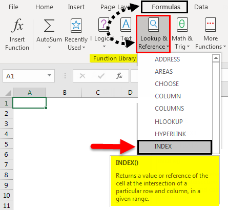
Using the INDEX function, we can find the value at the intersection of a specific row and column. The INDEX function in Excel is present under the Microsoft Excel Lookup and Reference function.
Key Highlights
- The INDEX function in Excel helps to find the information within a data range, where it looks up values by both columns and rows.
- It looks up the value of a cell at the intersection of a given row and column.
- We use the INDEX function in Excel with the MATCH function more commonly. The combination of the INDEX and MATCH functions is an alternative to the VLOOKUP function, which is more powerful & flexible.
- We can use the INDEX function in Excel to fetch individual values or entire rows and columns.
INDEX Function in Excel Syntax
There are two types of the INDEX function in Excel:
#1 Array Form
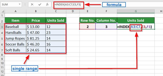
We use the Array INDEX form when the cell we refer to is within a single range of the data table, e.g., A3:C7.
To understand better, refer to the below image-
Syntax-
#2 Reference Form
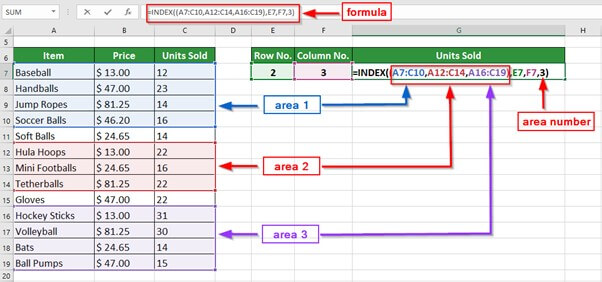
We use this INDEX form when the cell that we are referring to is within multiple cell ranges, e.g., (A7:C1,A12:C14,A16:C19)
Refer to the below image-
Syntax-
Explanation of the Syntax
array:
It is a compulsory or required argument that indicates the range or array of cells we want to look up
Note: If there are multiple cell ranges in the data table, it is called a reference where all the cell ranges(areas) are separated by a comma and with closed brackets
row_num:
It is a compulsory or required argument that indicates the row number against which we want to fetch the value.
Note: Excel considers the row_num argument optional if only one row exists in an array or cell range.
col_num:
It is a compulsory or required argument that indicates the column number against which we want to fetch the value.
Note: Excel considers the col_num argument optional if only one column exists in an array or cell range.
area_num:
It is an optional argument. If the desired value is present in multiple cell ranges in the data table, the area_num indicates the cell range to use.
Note: If there is no value in area_num, then by default, the INDEX Function in Excel considers the first area as the area number.
How to Use the INDEX Function in Excel?
To understand the usage of the INDEX function, consider the below-given examples.
ARRAY FORM
Example #1:
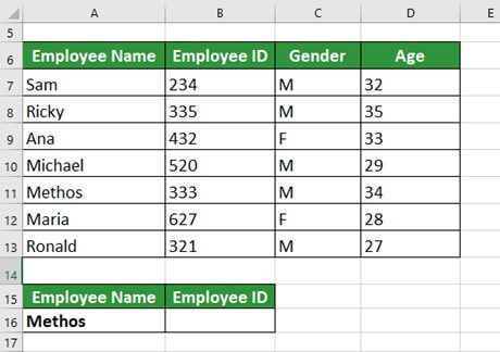
The table contains the name of Employees of a company, their Employee ID, Gender, and Age. We want to find the Employee ID of Methos using the INDEX function.
Solution:
We will apply the INDEX formula in cell B16 to get the Employee ID of Methos.
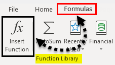
Step 1: Click on the Insert Function (fx) option under the Formulas section of the Excel toolbar.
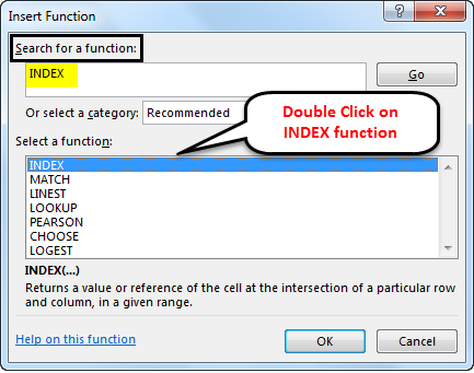
An Insert Function dialog box appears.
Step 2: Type INDEX in the dialog box’s Search for a function option. And double click the INDEX option from the list.
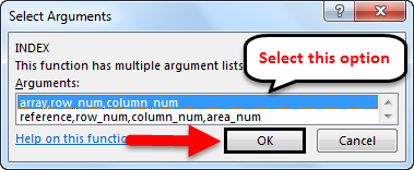
A Select Arguments dialog box shows the two types of INDEX functions: one for array and the other for reference.
Step 3: Select the array formula, as we have only one data range, and click OK.
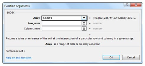
A Function Arguments dialog box opens with options Array, row_num, and column_num.
Step 4: Enter the cell range (A7:D13) that contains the lookup value in the Array argument
Note: Do not select the column headings
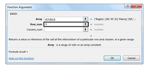
Step 5: Enter the row number(5) that contains the lookup value in the row_num argument.
Step 6: Enter the column number(2) that contains the lookup value in the Col_num argument.
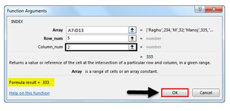
Step 7: Click OK to get the below result
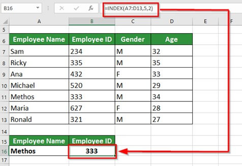
The Index function will return the value of the 5th row and 2nd column, i.e., Employee ID 333.
Example #2
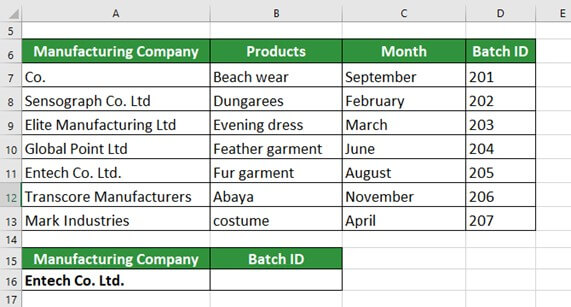
The table below shows the Batch ID of Clothing products manufactured by different industries. We want to find the Batch ID of products manufactured by Entech Co. Ltd.
Solution:
Step 1: Write Entech Co. Ltd. in cell A16
Step 2: Place the cursor in cell B16 and enter the formula,
=INDEX(A7:D13,5,4)
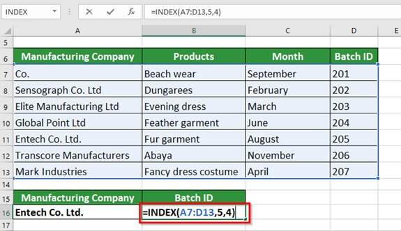
Explanation:
A7:D13: It is the cell range that contains data about Entech Co. Ltd.
5,4: The lookup value- Entech Co. Ltd. is in the 5th row of the selected cell range with Batch ID in the 4th column.
Therefore, we write 5 & 4, respectively, in the formula.
Step 3: Press the Enter key to get the below result
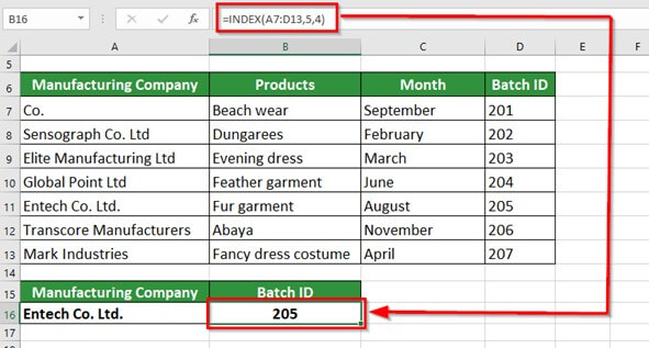
The INDEX function with Array Form gives the Batch ID of 205 for products manufactured by Entech Co. Ltd.
Example #3
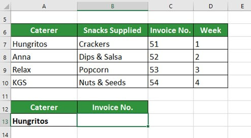
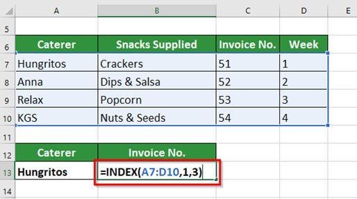
The table below shows 4 different caterers with snacks they supplied and invoice numbers for their respective bills. Here, we want to find the invoice number for the bill of the snacks supplied by Hungritos.
Solution:
Step 1: Write Hungritos in cell A13
Step 2: Place the cursor in cell B13 and enter the formula,
=INDEX(A7:D10,1,3)
Explanation:
A7:D10- It is the cell range that contains the data of Hingritos.
Note: We do not select the headings of the table.
1,3- The lookup value- Hingritos is in the 1st row of the selected range with invoice no. in the 3rd column. Therefore, we write 1 & 3, respectively, in the formula.
Step 3: Press the Enter key to get the below result
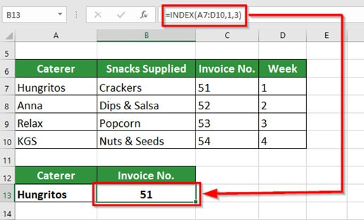
The INDEX function returns invoice no. 51 for snacks provided by Hungritos.
REFERENCE FORM
Example #1
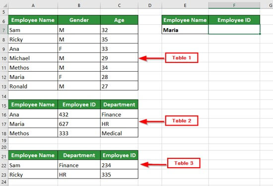
The table below shows three different tables with Employee Name, Employee ID, Gender, Age, and Department. We want to find the Employee ID of Maria using the INDEX function in Excel.
Solution:
Here, we will use the Reference Form of Excel since there are three different data tables.
Step 1: Write Maria in cell E7
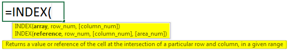
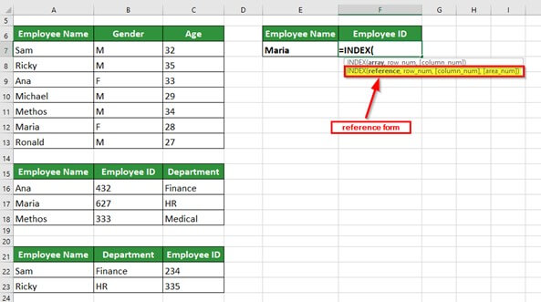
Step 2: Place the cursor in cell F7 and type =INDEX(
When we type the above, it displays two arguments, as shown in the image below
Step 3: Enter the formula,
=INDEX((A7:C13,A16:C18,A22:C23),2,2,2)
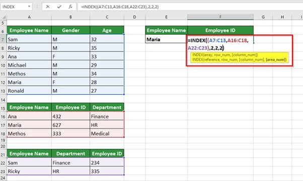
- Row_num: It is the row against which we want to fetch the Employee ID of Maria present in table 2; therefore, we enter row number(2), the intersection will occur at the 2nd row of the table
- Col_num: It is the column against which we want to fetch the value, i.e., 2, the intersection will occur at the 2nd column of the 2nd table
- Area_num: It indicates the area(table) which contains the details of Maria, i.e., table 2. Thus, we enter the Area_num as number 2 here.
Step 4: Press the Enter key to get the below output
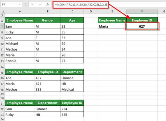
The INDEX function in Excel returns Employee ID of Maria as 627.
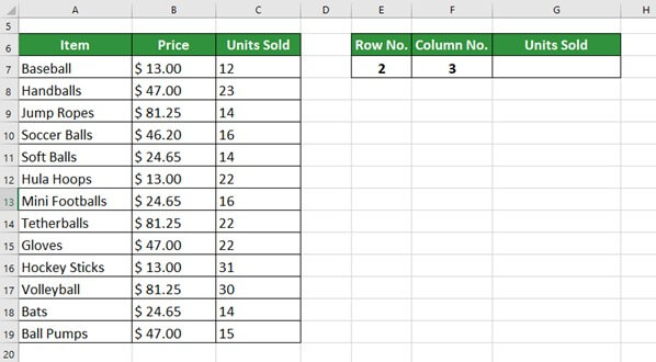
Example #2
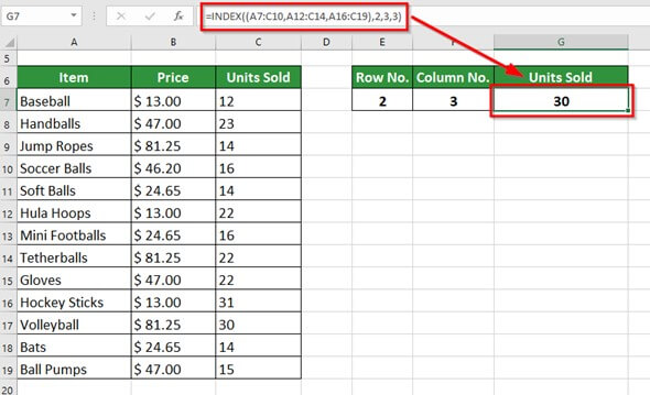
The table below shows sports items sold by a store with their prices. We want to find the number of Volleyballs sold by the store given the row number and column number.
Solution:
Step 1: Write the desired row and column numbers in cells E7 and F7, respectively.
Step 2: Place the cursor in cell G7 and enter the formula,
=INDEX((A7:C10,A12:C14,A16:C19),2,3,3)
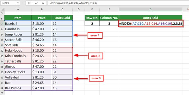
The table above has three different areas- area 1, area 2, and area 3. Our desired item, a Volleyball, is in the third area. Therefore, we write the number 3 at the end.
Step 3: Press the Enter key to give the below result.
Things to Remember
- The INDEX function in Excel returns #VALUE! Error if row_num/ column_num is not mentioned in the formula or given as 0.
- The INDEX function returns #VALUE! error if the values for row_num, col_num, or area_num are non-numeric.
- The INDEX function in Excel returns #REF! Error if the value entered for row_num exceeds the number of rows present in the data table
- The INDEX function returns #REF! Error if the value entered for column_num exceeds the number of columns present in the data table
- The INDEX function in Excel returns #REF! Error if we provide a value for area_num greater than the number of areas in the cell range.
- If we give (refer) the area_num in the INDEX Formula from another sheet, the Index Function in Excel returns #VALUE! Error. It should represent the table present in the same sheet.
Frequently Asked Questions (FAQs)
Q1) What is the use of INDEX ()?
Answer: With the INDEX (), we can find the index position of an element or character in an item string. It gives the lowest possible index of the specified element in the list. If the provided item is not in the list, the INDEX function in Excel returns a ValueError.
Q2) What is the INDEX formula?
Answer: The INDEX formula for the Array form is
=INDEX(array, row_num, [col_num]).
The INDEX formula for Reference form is =INDEX(reference,row_num,[column_num],[area_num]).
The array argument specifies the cell range we want to look up. If there are multiple cell ranges in the data table, we separate them using a comma and close them with brackets; row_num indicates the row number against which we want to fetch the value; col_num indicates the column number against which we want to fetch the value; area_num indicates the range to use if there are multiple areas(tables).
Q3) What is the purpose of the INDEX and MATCH functions?
The INDEX function provides the value of a parameter based on the row and column numbers. The MATCH function gives the position of a cell in a column or a row. Combining the INDEX and MATCH functions provides a cell value based on horizontal and vertical criteria.
Recommended Articles
The article is a guide to the INDEX Function in Excel. Here we discuss how to use the INDEX Function in Excel, with practical examples and a downloadable excel template. Enhance your knowledge with these useful functions in excel
