Updated July 3, 2023
What is VLOOKUP in Excel?
VLOOKUP Function in EXCEL stands for Vertical Lookup. It is an Excel function to find specific information in a vertical pattern across a table or Excel spreadsheet.
The below image shows the Lookup column and Result column that Vlookup will use to scan and display the result.
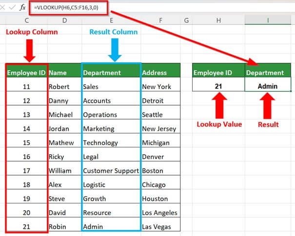
For example: Consider a database with an employee ID, name, work department, and location. You want to check the employee’s work location with employee ID 12. Rather than doing it manually, you can apply the VLOOKUP formula to automate the process.
We can use the formula =VLOOKUP (A3, A2:D12, 4, 0) to find the required information.
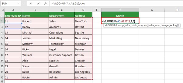
Cell A3 denotes the employee ID 12, the table array denotes the selected range in Red, and the column number indicates the selected column 4 for finding the address of the employee-Danny, against the employee name. Once you enter the VLOOKUP formula in the cell, hit the Enter key, and we will get the exact match.
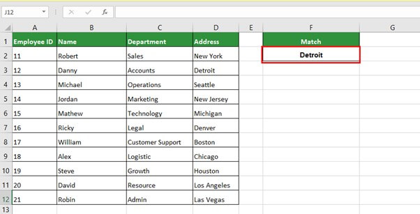
The image below shows the output, i.e., the address of Danny- Detroit.
Key Highlights
- In Vlookup Function in Excel, the V stands for vertical. The Vlookup function scans from the left and moves to the right of the data table.
- Vlookup scans for both exact and approximate matches of the looked-up value.
- When duplicate values are non-existent, we use them for a given data table, and if Excel finds duplication, the function returns only the first one.
- True implies an absolute, and false indicates an incorrect or close match.
VLOOKUP Syntax
Vlookup Arguments
There are four arguments in the Excel vlookup function, mentioned below:
- Lookup value (required): Excel indicates it as the lookup value when we need to work with an element. For example, the employee ID.
- table_array (required): It is the range containing the lookup value. For example, the data range has the employee ID, name, work department, and address.
- Col_ index_ num (required): When we wish to return a value or element from a table array, col_index_num specifies its column number. For example, The column number for finding the address is 4.
- range_lookup (optional): It is the fourth argument of the Vlookup formula. Range_lookup instructs Excel to return either an Exact or Approximate If we provide 0 or False, it will return an Exact match, and if we provide 1 or True, it will return an Approximate match to the looked-up value.
How to Use the VLOOKUP Function in Excel?
Let us understand the use of the Vlookup function with examples:
Example of VLOOKUP Function in EXCEL
1. Finding the Exact Match
The table below shows the Employee IDs and the Names, departments, and Addresses of company employees. We wish to find the Department of Persons with Employee ID 16.
Solution:
Follow the below steps to find the Department of Employee ID 16
Step #1: Organize the data in a table because the Excel function will automate its operations in the same manner
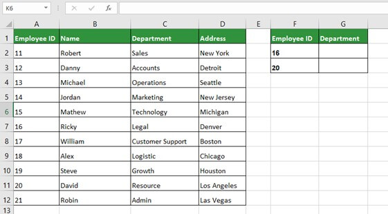
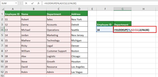
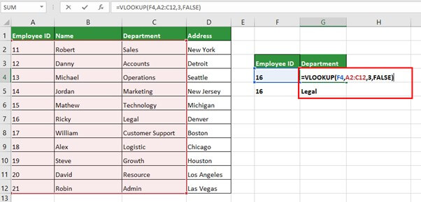
Step #2: Click on the cell G4 and Enter the lookup formula: =VLOOKUP(F4,A2:C12,3,FALSE)
In the above formula, F4 denotes employee ID, the table array is the highlighted range, and the column is an integer you select to get the looked-up value. The last value helps in returning the exact or approximate match.
- If True, it is an approximate match.
- If False, it is an exact match.
Below given image shows the entire Vlookup operation:
Step #3: Press Enter to see the result shown in the image below.
2. Finding Another Exact Match
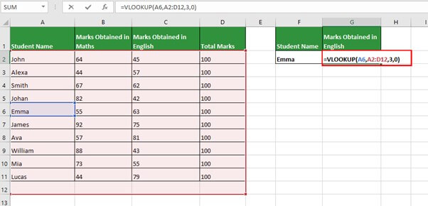
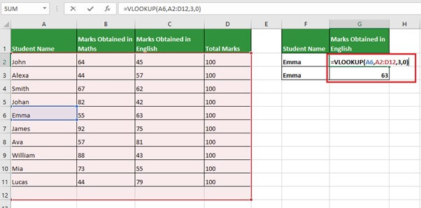
The following table shows students and their marks obtained out of 100 in English and Maths. We need to find scored marks of Emma in the English subject.
Solution:
Follow these steps to find marks of Emma in English.
Step #1: Organize the data from left to right
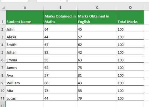
Step #2: Place the cursor in the G2 cell and enter the below-given formula,
=VLOOKUP(A6,A2:D12,3,0)
Step #3: Once you hit the Enter key, it will display the output, i.e., marks obtained in English by Emma, as shown in cell G3
3. Finding an Approximate Match
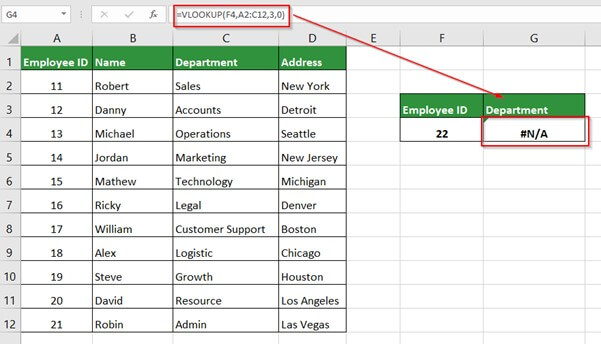
In this example, we wish to find the Department of Employee ID 22
Solution:
Follow the steps given below.
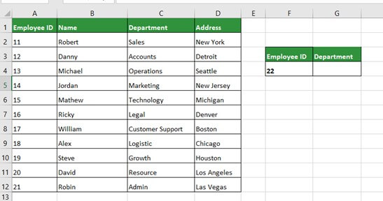
As per the data, we do not have the Employee ID of 22. So, we have to automate the process through an approximate match function.
The entire step is the same as the exact match function except for the lookup_range value.
Below are images to understand the same.
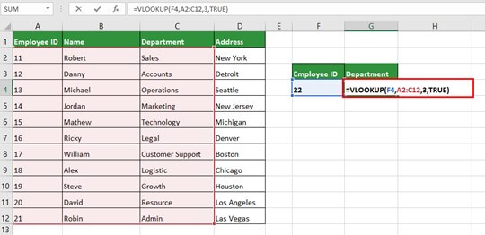
In the range_lookup function, we provide TRUE for the approximate match.
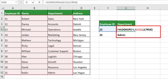
Once you press Enter key, Excel gives the output Admin. If the looked-up data is not in the table, Excel returns the relative value (approximate) to the previous value.
Explanation– The table does not have data about Employee ID 22. Thus, Excel will return the ID value just before ID 22, i.e., ID 21. The Department of Employee with ID 21 is Admin; hence the result for Employee ID 22 is also Admin.
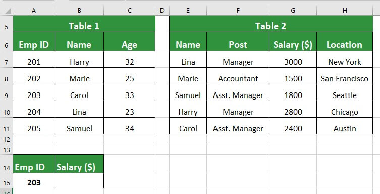
Nested VLOOKUP Function
If you have two tables that are not linked, you can use the nested VLOOKUP Function to find the information you need. The nested VLOOKUP formula searches for data that matches the lookup value in one of the tables. The output of this formula is then treated as the lookup value by the primary VLOOKUP function, which retrieves the relevant data from the second table.
Let’s say we have two tables. Table 1 contains the Employee ID, Name, and Age, while Table 2 contains Employee Name, Post, Salary, and Location. If we want to find the employee’s salary with ID 203 (in Table 1), we can use the nested VLOOKUP function to search for the corresponding information in Table 2.
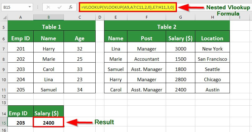
The Nested VLOOKUP formula that we will use here is: =VLOOKUP(VLOOKUP(A9,A7:C11,2,0),E7:H11,3,0)
The first VLOOKUP function, VLOOKUP(A9, A7:C11,2,0), searches for the value A9 (Emp ID 203) in Table 1 (A7:C11) to find the corresponding name from column 2.
The function returns the output as Carol.
The output is treated as the lookup value by the main formula. The first VLOOKUP function will search for Carol in the table range (Table 2) and provide the corresponding data (Salary) from column 3. Therefore, the output of the Nested VLOOKUP formula is $ 2400, which means the salary of a person with employee ID 203 is $ 2400.
Alternatives to VLOOKUP
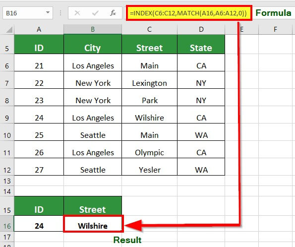
1. Index Match Function
It is a more efficient alternative to the VLOOKUP function in Excel. It is faster, does not require sorting the lookup array, and returns a reference to a cell rather than a value. This makes the Index Match function ideal for working with large datasets.
For example, if you need to find the street with ID 24, use the Index-Match function, as shown in the image below.
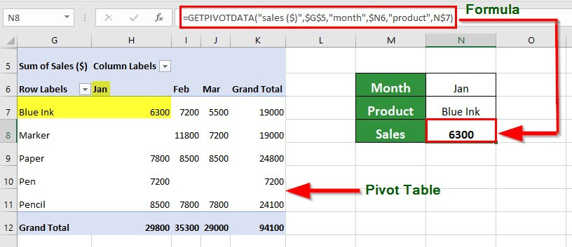
2. GETPIVOTDATA Function
Although the VLOOKUP function can retrieve information from Pivot Tables, it can be limited in its functionality. If the table is modified, the VLOOKUP formula may not work correctly.
Fortunately, Excel has a built-in function called “GETPIVOTDATA,” which can help in such cases. Unlike VLOOKUP, the GETPIVOTDATA function does not rely on cell ranges to look up values. Instead, it uses specific criteria to return accurate results, even if the table changes.
For instance, if you want to find the sales of a product in a specific month from a Pivot Table, you can use the GETPIVOTDATA function. The image below shows how you can use the function to retrieve the desired data.
Real-World VLOOKUP Applications
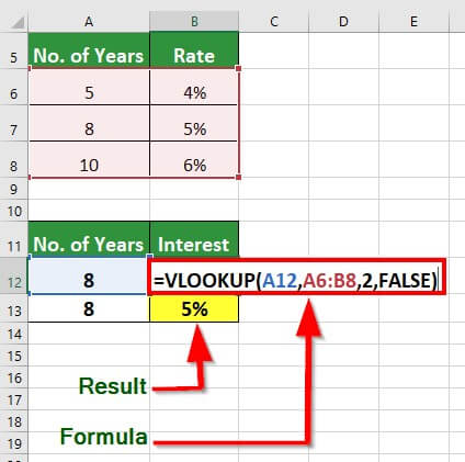
1. Financial Modeling
We can use VLOOKUP to make financial models more dynamic by retrieving information based on multiple scenarios. For instance, consider a financial model that includes a loan repayment schedule. A company levies a different interest rate based on the total years a person takes to repay the loan: 4.0 %, 5%, and 6%. We can use VLOOKUP to obtain the corresponding interest rate for each repayment period. It makes the financial model more flexible as it can easily factor in multiple variables and scenarios.
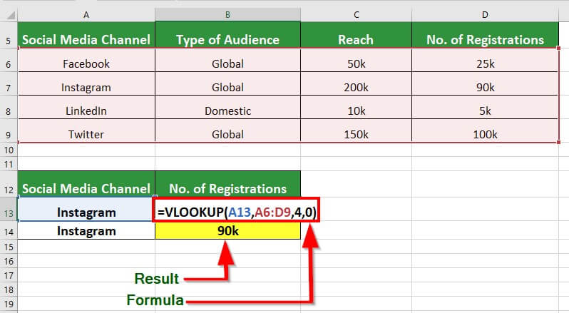
2. Marketing
A marketing agency can use VLOOKUP to determine the impact of its marketing campaigns. For instance, if a firm announces a free online event on multiple social media channels, it can use VLOOKUP to calculate the number of registrations for the event from each platform. This easy, the agency can identify which platforms are generating the most signups.
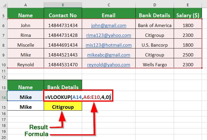
3. Human Resource
When managing employee information, VLOOKUP is a common tool used in many organizations, particularly in Human Resource departments. Consider a table that lists employee details, such as their name, contact number, email ID, bank details, and salary. To transfer an employee’s salary, you can use VLOOKUP to retrieve their bank details with ease and accuracy.
Excel Vlookup Errors
- #N/A!: Excel gives this error when the Vlookup function cannot find lookup_value in the table_array.
- #REF!: This error occurs when we provide a column number (col_index_ num) more than the number of columns in the data table (table_array).

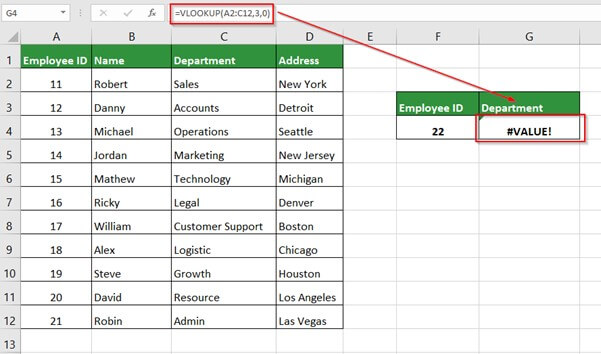
- #VALUE!: Excel gives this error when we do not provide the column number (col_index_ num), or we have given a value less than 1.
VLOOKUP Add-ons
Add-ons are additional functionalities of Excel that we can combine with VLOOKUP to produce more accurate results and increase efficiency.
1. Power Query
This add-on allows us to work with data in any order or format without organizing it in a specific way for VLOOKUP. Power Query can merge data tables and find a common column to provide the required information from the lookup column. It also stores the steps performed in memory, which can be helpful for refreshing data later.
2. Power Pivot
With Power Pivot, we can add columns to a dataset without creating new VLOOKUP formulas. This add-on works by creating relationships between multiple tables. It makes it easier to look up values from a particular table and fetch the corresponding information from another table.
3. Fuzzy Lookup Add-in
We can use this add-in to compare two similar data columns and provide a table of matched identical data. However, it cannot fetch exact matches, only similar data.
4. Essential Excel Add-In
This add-in is written in VBA and uses User Defined Functions to simplify the VLOOKUP operation. It can return data from any column, regardless of its order in the data set.
VLOOKUP in Other Spreadsheet Applications
We can use VLOOKUP in other spreadsheet applications such as Google Sheets and Apple Numbers. It works as it does in Excel, i.e., looking up vertically in a data table to find the value in the query and returning the corresponding information.
1. VLOOKUP in Google Sheets
The syntax for VLOOKUP in Google Sheets is =VLOOKUP(search_key, range, index, [is_sorted])
- Search_key is the lookup value
- range which is the data set containing the search key. The corresponding data
- index is the column number containing the required data
- is_sorted is an optional argument and requires a 0 for an exact match and 1 for an approximate match.
2. Apple Numbers
The syntax for VLOOKUP in Apple Numbers is: VLOOKUP(search-for,columns-range,return-column,close-match)
- Search-for is the lookup value
- columns-range, as the name suggests, is the range containing lookup value and related information
- return-column is the column number containing the required data
- close-match requires a False for the exact match and a True for the approximate match.
Comparison Table
|
Particulars |
Microsoft Excel | Google Sheets |
Apple Numbers |
| Syntax | VLOOKUP(lookup_value, table_array, col_index_num, [range_lookup])
|
VLOOKUP(search_key, range, index, [is_sorted]) | VLOOKUP(search-for,columns-range, return-column,close-match) |
| Tables
|
The lookup value must be in the same data table | Google Sheets lookup value can be in a different data table | The lookup value can be in another data table |
| Supports wild card characters? | Yes | Correct, but it can result in inaccurate output | Yes, but it can result in erroneous output |
VLOOKUP vs. HLOOKUP
|
Particulars |
VLOOKUP |
HLOOKUP |
| Meaning | It stands for vertical lookup. | It stands for horizontal lookup. |
| Use | It searches for data in a vertical pattern across the columns and returns the corresponding information. | It searches for data in a horizontal pattern across the rows and returns the corresponding information. |
| Popularity | It is a popular Excel function for financial operations. | It is less popular among users. |
| Tables | It finds data from the leftmost columns of the tables to the right. | It finds out data from the top to the bottommost rows of tables. |
| Output | The output is the same for both functions. | There is no difference in the outputs. |
Things to Remember
- VLOOKUP always returns the first value it finds upon searching across all columns.
- It only looks for data on the right side of the lookup column, whether the lookup column is at the beginning or middle of the sheet.
- It is not case-sensitive, working the same for lowercase, uppercase, and letters as long as the syntax is correct.
- Use named ranges in the VLOOKUP formula to ensure Excel does not adjust the reference if you copy the formula to another cell or worksheet.
- Avoid hardcoding in formulas. For example, consider writing days_in_a_month instead of 30 or 31.
- Use Ctrl + Shift + Enter key instead of pressing the simple Enter key to fetch values from multiple columns in one go. It will save calculation time and increase speed.
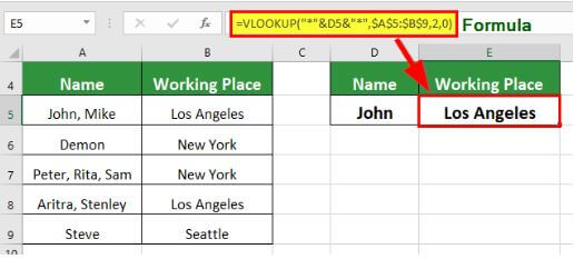
- Use Wildcard characters in the VLOOKUP formula to get the required data whenever we change the lookup value in the table. For example, cell D8= cherry, and we want to find its price from table range A1:C6. The formula =VLOOKUP(“*” &D8&”*”, A1:C6,2, FALSE) will provide the corresponding cost of fruit.
Frequently Asked Questions (FAQs)
Q1. How to use the VLOOKUP function in Excel to find a partial match?
Answer: To use the VLOOKUP function for finding a partial match, we have to combine the wildcard character (*) asterisk with the lookup_value as shown below-
=VLOOKUP(value& “*”, data,2, FALSE)
Q2. How can the VLOOKUP Excel formula be applied for absolute and relative cell references?
Answer: When working with Excel sheets, we often want the lookup range to remain the same. To lock the range, we use absolute references by inserting dollar $ before each part of the reference as shown below-
=VLOOKUP(C3,$J$3:$L$11,2,true)
Excel uses relative cell reference when we apply the same formula to more cells. We copy the formula and paste it into the desired cell. Here, Excel automatically changes the values of lookup_value and table_array as per the original formula.
For example,
=VLOOKUP(F4,A2:C12,3,0) is the original formula
=VLOOKUP(F5,A3:C13,3,0) is the copied formula. Here Excel has changed the lookup_value and table_array as per the looked-up value.
Q3. What is the importance of the VLOOKUP function?
Answer: We use the VLOOKUP function to find specific information from a large data set. VLOOKUP works like a phone book, where you find the phone number of a person using their names in the phone book. When working on large data sets, Vlookup is a time-saving tool.
Q4. Does VLOOKUP work in google sheets?
Answer: VLOOKUP is very efficient in Google Sheets when dealing with interrelated data across many tables. However, it does not accept more than 255 characters for a single value argument in Google Sheets.
Q5. When would you use an HLOOKUP instead of a VLOOKUP?
Answer: HLOOKUP stands for horizontal lookup. It helps to look up data arranged in rows. On the other hand, VLOOKUP, short for vertical lookup, searches for data arranged in columns.
Q6. Is VLOOKUP case-sensitive?
Answer: No, VLOOKUP is not case-sensitive. VLOOKUP will search for the data, regardless of using uppercase and lowercase letters, as long as the syntax is correct.
Recommended Articles
The above article is EDUCBA’s guide on using the Vlookup function in Excel. Learn more by visiting these Recommended Articles:
