Updated October 18, 2023
What is HLOOKUP in Excel?
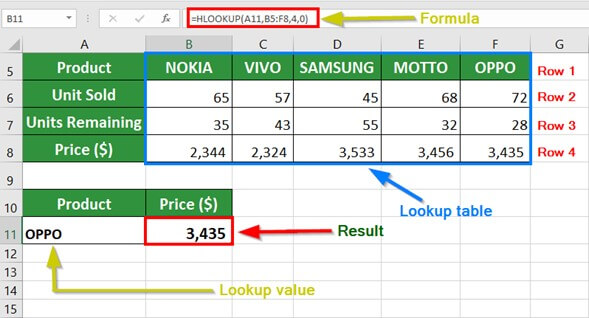
The HLOOKUP function in Excel performs a horizontal search across a sorted data table to find a match with the lookup value. It searches across the topmost row for the look-up value and then moves down to retrieve data from the specified row.
In HLOOKUP, the H stands for Horizontal, which we use when the lookup table is arranged horizontally. We can use the function to search for numbers, text, or logical values.
For example, =HLOOKUP(A11, B5:F6,4,0) scans the lookup table to find the price of OPPO and gives the result of $3,435.
Key Highlights
- In the HLOOKUP in Excel, “H” stands for horizontal. The HLOOKUP function scans from the top and moves to the last row of the data table.
- HLOOKUP scans the data table for exact and approximate matches of the looked-up value.
- If HLOOKUP in Excel finds duplication in the data range, the function returns only the first match.
- TRUE in the HLOOKUP argument indicates an absolute match, and FALSE indicates a close match.
Syntax of HLOOKUP in Excel
The syntax for the HLOOKUP function is-
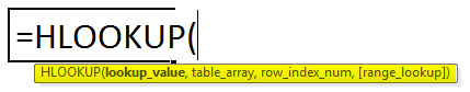
- Lookup_Value: It is the Base Value or Criterion Value to search in the table.
- Table_Array: It is the table range in which the targeted value resides.
- Row_Index_Num: It represents the row number where the targeted value is present. The first row is entered as 1, the second as 2, and so on.
- [Range_Lookup]: It consists of two parameters- TRUE or 1 searches for an approximate match in the data table; FALSE or 0 looks for an exact match.
How to Use HLOOKUP in Excel?
To understand the use of HLOOKUP, consider the following examples:
Example #1
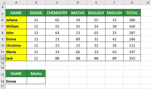
The table below shows students’ marks in Grade 12 in the subjects- Chemistry, Maths, Biology, and English. We want to find the marks scored Emma in Maths using the HLOOKUP function.
Solution:
Step 1: Place the cursor in cell B16 and type the formula,
=HLOOKUP(B15,A5:G12,5,0)
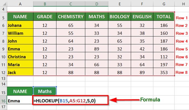
Explanation:
- B15: It is the look-up value (Maths)
- A15:G12: It is the cell range from which HLOOKUP will search the marks
- 5: It indicates the row number from which Excel needs to fetch data
- 0: It indicates that we want the Exact match
Note: We can use FALSE or 0 to indicate an Exact match.
Step 2: Press Enter key to get the below result
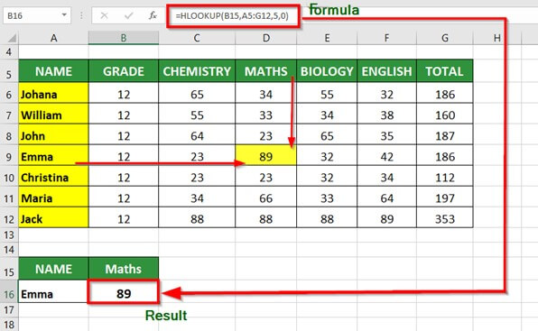
The HLOOKUP function displays that Emma scored 89 marks in Maths.
Example #2
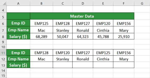
The table below shows master data consisting of Employee ID, Employee Name, and Salary. We want to find the salary of all the employees using HLOOKUP in Excel.
Solution:
Step 1: Place the cursor in cell B13 and enter the formula,
=HLOOKUP(B11,$B$6:$F$8,3,FALSE)
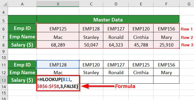
Step 2: Press Enter key to get the below result
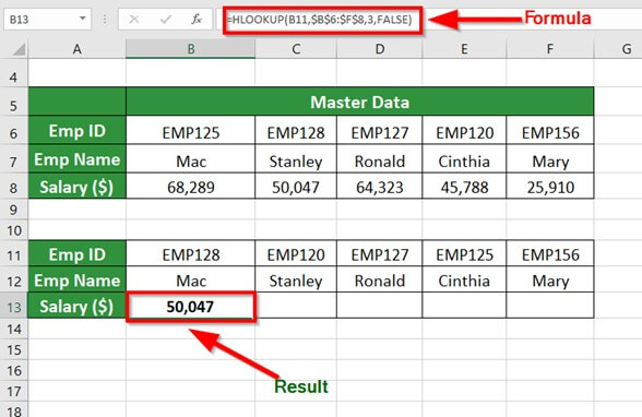
The HLOOKUP function gives a salary of $50,047 against Emp ID 128.
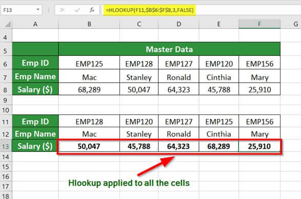
Step 3: Drag the formula in other cells to get the below result
Using HLOOKUP and MATCH Function Together
We use the Match function to look up multiple values from a data table. Whenever we change the look-up value, the Match function fetches the corresponding row number for HLOOKUP to give accurate results. In other words, we use the Match function when the row number is dynamic.
Consider the below example to understand the working of the Match function
Example #1
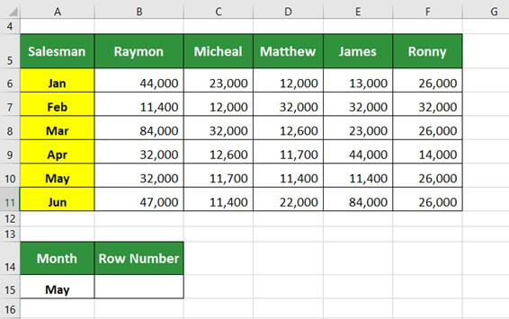
The below table shows the sales figures of 5 salespeople for Jan, Feb, Mar, Apr, May, and Jun. We want to find the row number for the month “May” using the MATCH function.
Solution:
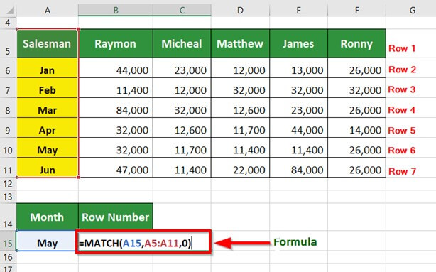
Step 1: Place the cursor in cell B15 and enter the formula,
=MATCH(A15,A5:A11,0)
Step 2: Press Enter key to get the below result
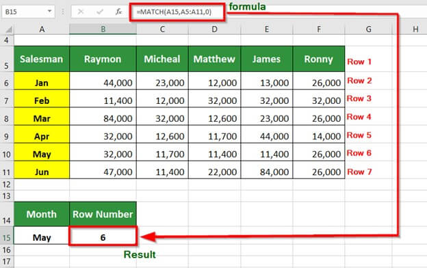
The MATCH function searches for A15 (May) in the column range A5:A11 and provides its row number of 6.
Example #2
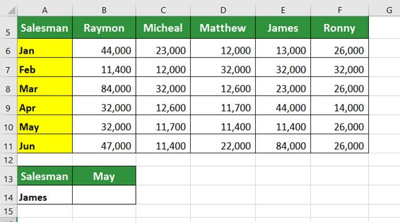
The below table shows the sales figures of 5 salespeople for Jan, Feb, Mar, Apr, May, and Jun. We want to find the sales figure of James in May using the HLOOKUP and MATCH functions.
Solution:
Step 1: Place the cursor in cell D16 and enter the formula,
=HLOOKUP(C16,C7:H13,MATCH(D15,C7:C13,0),0)
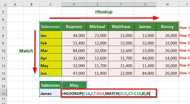
Explanation: The HLOOKUP searches for C16 (James) in the range C7:H13
The MATCH function searches for D15 (May) only in the C column in the data range C7:C13 to give the row number 6. Therefore, HLOOKUP fetches the sales figure of James from row 6.
Step 2: Press Enter to get the below result,
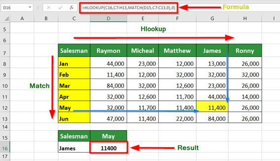
The HLOOKUP and Match function provides the sales figure of 11400.
HLOOKUP in Excel Errors
The HLOOKUP function displays the following Errors:
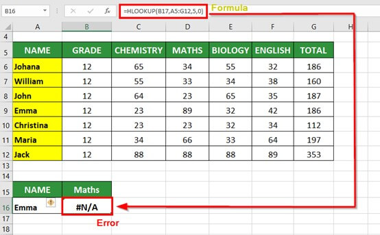
- #N/A!: Excel gives this error when the HLOOKUP function cannot find the lookup_value in the table_array.
For example,
Cell B17 (lookup value) in the table below contains no data. Therefore, HLOOKUP displays the error #N/A!
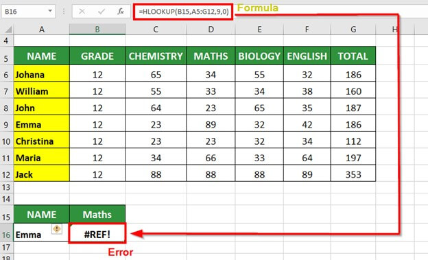
- #REF!: This error occurs when we provide a row number (row_index_ num) greater than the number of rows in the data table (table_array).
For example,
In the table below, the row number (9) we have provided in the formula is greater than the table’s number of rows. Therefore, HLOOKUP displays the error #REF!
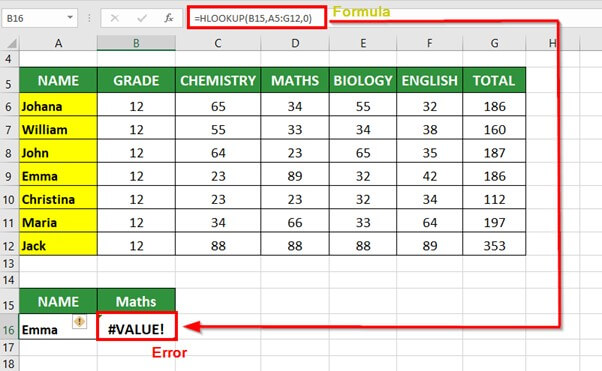
- #VALUE!: Excel gives this error when we do not provide the row number (row_index_ num), or we have given a value less than 1.
For example,
In the below table, we have not provided the row number in the formula. Therefore, HLOOKUP displays the error #VALUE!
Frequently Asked Questions (FAQs)
Q1) Is HLOOKUP better than VLOOKUP?
Answer: VLOOKUP and HLOOKUP are useful when finding data in a large database with many rows and columns. However, both HLOOKUP and VLOOKUP have advantages and disadvantages.
We can use Vlookup only when the lookup value is in the first column and HLOOKUP when the look-up value is in the first row of the data table. The functions fail to give accurate results when the data set has duplicate values.
Q2) What is the syntax of HLOOKUP?
Answer: The syntax of HLOOKUP is:
=HLOOKUP(lookup_value, table_array, row_index_num, range_lookup)
- Lookup_value: The value you want to find in the 1st row of the cell range.
- Table_array: It is the table that contains lookup data. It is important to ensure the lookup data is in the top row of the table array.
- row_index_num: It is the row containing the desired value.
- [range_lookup]: It requires FALSE or 0 to provide an exact match to the look-up value and TRUE or 1 for an approximate match.
Q3) How do I use HLOOKUP in sheets?
Answer: To use HLOOKUP in Google Sheets, consider the below example to find the number of apples sold on Day 4.
Step 1: Select the cell where you want the result
Step 2: Place the cursor and type the formula
=HLOOKUP(“Apple”,B1:E6,5,0)
Step 3: Press Enter key to get the result of 16
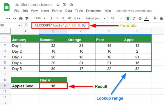
The HLOOKUP searches for the lookup_value (Apple) in the table range B1:E6, moves horizontally to row number 5 and provides the value of 16.
Or,
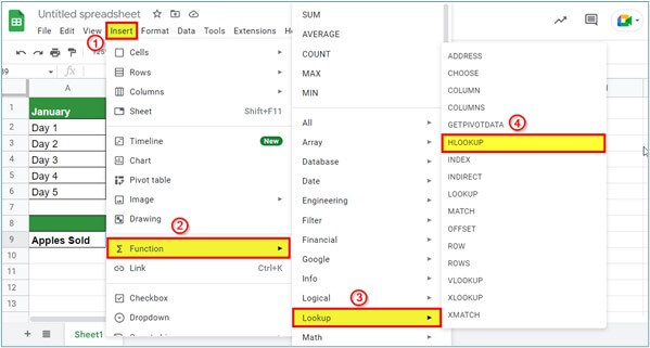
We can also locate the HLOOKUP function in Google Sheets using the Insert menu,
Insert > Function > Lookup > HLOOKUP.