Why Learn About Advanced Excel Formulas and Functions?
In today’s world, almost every business, however big or small, uses software and tools to run smoothly and effectively. Among various tools, Microsoft Excel is the most common, efficient, and important tool. Companies mainly choose Excel because of the advanced formulas and functions that help them solve most complex tasks in a second.
While the main application of Excel is to help you store and maintain data, advanced Excel functions help you understand your data, perform difficult calculations, and even make automated decisions. If you own a business, you can use advanced formulas in Excel to prepare budgets, sales reports, balance sheets, editorial calendars, and so much more. On the other hand, you can also use these formulas for personal purposes, like tracking expenses, planning day-to-day tasks, managing debt payments, etc.
These Excel formulas can save you time by giving faster and more accurate results, but only if you know how to use them correctly. So, it is important that you know the common advanced functions in Excel and when and how to use them.
So, to help you, this article has the top 25 advanced Excel formulas list along with their syntax, uses, and examples.
Table of Contents
- VLOOKUP Function
- XLOOKUP Function
- IFERROR Function
- INDEX Function
- MATCH Function
- OFFSET Function
- SUMPRODUCT Function
- SUMIF Function
- COUNTIF Function
- IF combined with AND/OR Formula
- LEFT, MID, and RIGHT Functions
- CONCATENATE Function
- TRIM Function
- LEN Function
- CONVERT Function
- SORT and SORTBY Functions
- REPLACE and SUBSTITUTE Functions
- CHOOSE Function
- WORKDAY and NETWORKDAYS Functions
- PV Function
- PMT Function
- ROUND Function
- UNIQUE Function
- ISNUMBER Function
- Goal Seek Function
Top Advanced Excel Formula and Functions
1. VLOOKUP Function
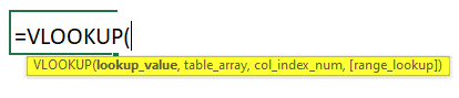
VLOOKUP in Excel stands for Vertical Lookup. VLOOKUP function searches for specific values (vertically) in a column and retrieves exact or approximate matches from another column from the same row.
Vlookup Syntax:
When to use it?
- Find product price based on product code
- Find a city based on its zip code
- Get the employee’s ID based on name
- Find commission based on sales, etc.
Example:
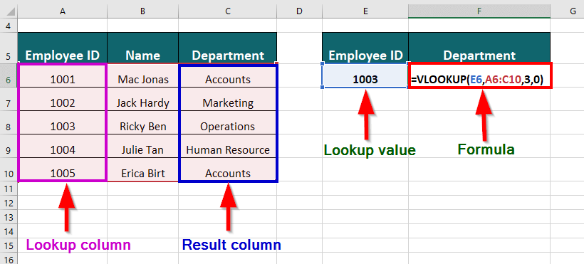
You have a table with a list of Employee_IDs, Employee_Names, and their departments and need to find the department of employee ID 1003.
You can use the VLOOKUP function to find the department of employee ID 1003:
The formula for VLOOKUP will be:
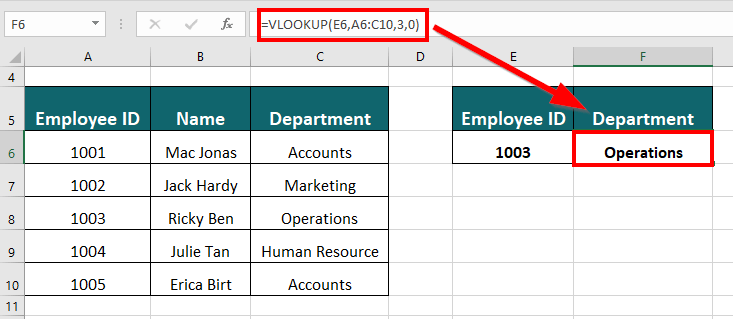
Result: The VLOOKUP formula will display “Operations”.
More advanced applications of the VLOOKUP function:
2. XLOOKUP Function
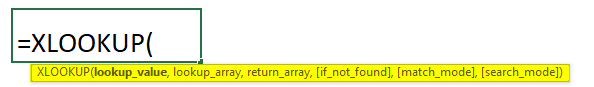
XLOOKUP function in Excel searches for lookup value vertically and horizontally in the table or array and returns the result from the same row.
XLOOKUP Syntax:
When to use it?
- To search the contact number of a particular customer
- To find the city name based on the pin or zip code
- To search the salary of employees based on their ID
- To see sales of specific products, etc.
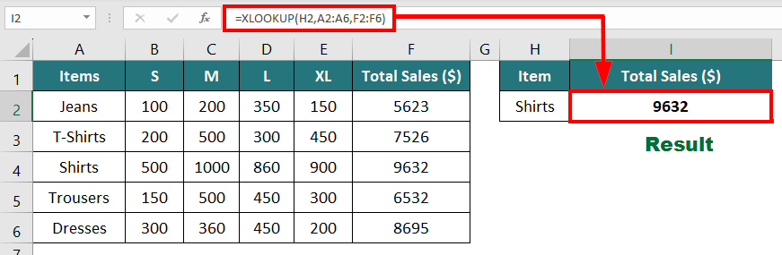
Example:
Suppose you have the following sales data for different clothing items and need to find the total sales of shirts.
The formula will be:
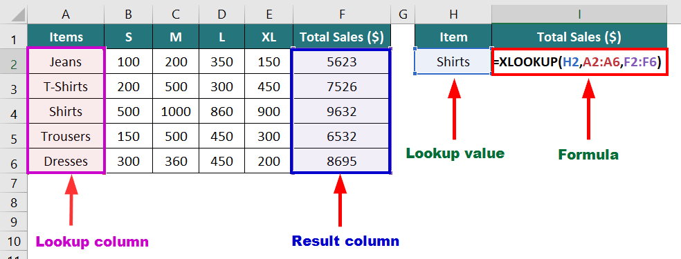
Result: The formula displays “9632”, i.e., total sales of shirts.
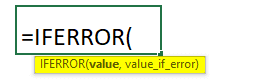
3. IFERROR Function
The IFERROR function in Excel is useful for returning a custom message when a formula gives an error.
IFERROR Syntax:
When to use it?
- To display “Invalid Data” instead of #VALUE!
- To display “Check Divisor” if the divisor value is zero or empty, etc.
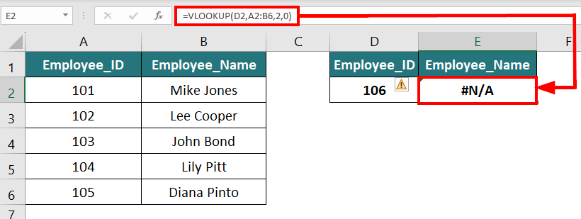
Example:
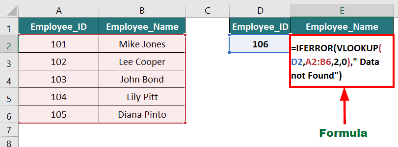
Suppose you use the VLOOKUP function to search for an employee’s name based on their employee ID. If that ID is not in the data table, it will display an #N/A error. Here, if you want to show a custom message instead of an error, you can use the IFERROR function.The formula to add a custom message will be:
The below image shows what will happen if we don’t use the IFERROR function.
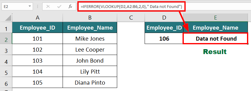
Now, let us use the IFERROR function.
Result: The formula displays “Data Not Found” instead of an error.
More advanced applications of the IFERROR function:
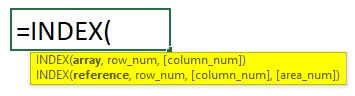
4. INDEX Function
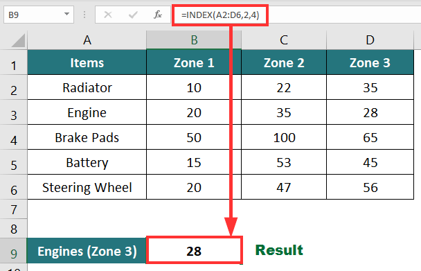
The INDEX function finds the cell where the specified row number and column number meet in the given range and then returns the value present in that cell.
INDEX Syntax:
When to use it?
- To get a student’s grade for a particular subject
- To retrieve a product’s sales revenue for a particular region, etc.
Example:
If we want to retrieve the number of engines sold in Zone 3 from the below data,
You can use the following formula:
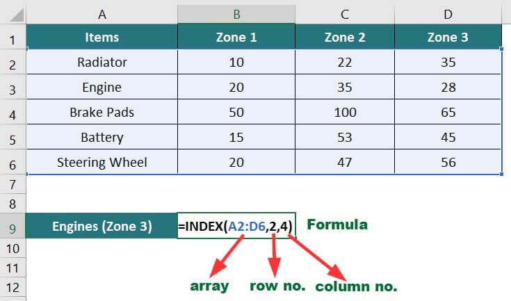
Result: The formula displays “28”, no. of engines sold in Zone 3.
More advanced applications of the INDEX function:
5. MATCH Function
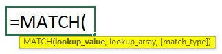
The MATCH function in Excel returns the position of the given value in a row or column.
MATCH Syntax:
When to use it?
- To find the exact position of a customer’s contact no. from a list
- Using a student’s name to find the row where the student’s details are present
- To find the “Out of stock” item to check inventory status, etc.
Example:
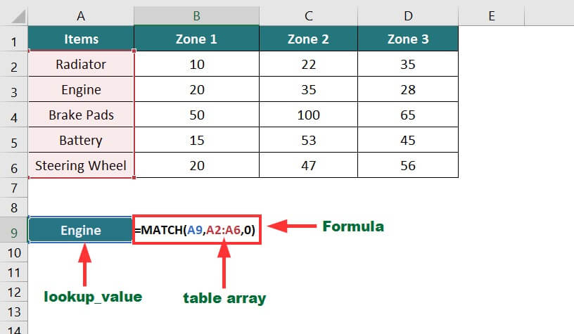
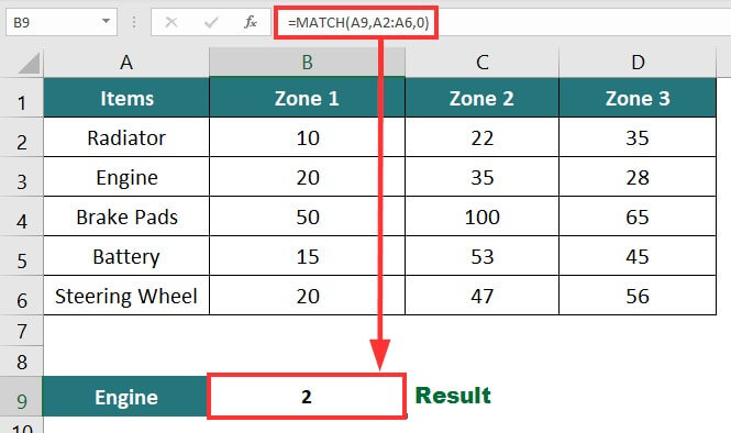
In the below data, we want to know the position of the word “Engine” in the “Items” column.
The formula for that will be:
Result: The formula displays “2”, i.e., the engine’s position in the table.
6. OFFSET with SUM Function
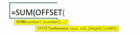
The OFFSET function in Excel returns a value or cell range using the reference cell we enter as a starting point. For example, if the formula is =OFFSET(A1, 4,1), the function will move 4 rows below from A1, i.e., A4 and 1 column to the right, giving us the value in B5. We can use the OFFSET function with the SUM/AVERAGE functions for dynamic results.
OFFSET combined with SUM Syntax:
When to use it?
- To calculate the total expense of specific months
- To change the seating plan for an event due to an unexpected change in the guest list
- To retrieve important data from a large dataset, etc.
Example:
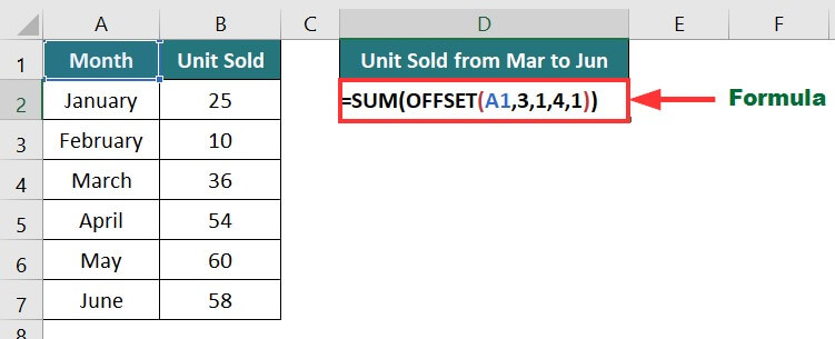
In the below data, we need to calculate the unit sold from March to June using SUM and OFFSET functions.
The formula for calculating total units will be:
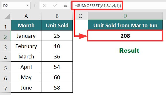
Result: The formula returns “208”, i.e., the total unit sold from March to June.
Explanation: =SUM(OFFSET(A1,3,1,4,1))
The OFFSET function starts from Cell A1 (Reference cell), moves 3 rows down, 1 column right, and reaches Cell B4. The SUM function adds the values of 4 cells below, including B4 (B4:B7), and returns 208.
More advanced applications of the OFFSET function:
7. SUMPRODUCT Function
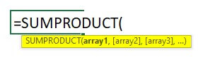
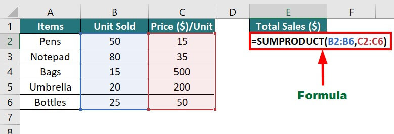
The SUMPRODUCT function multiplies each value in one column by the corresponding value in a second column, then adds all the multiplied values and returns the final result. It performs two important calculations in a second, saving us much time.
SUMPRODUCT Syntax:
When to use it?
- To calculate total sales for a year using quantity sold and price per unit
- To find your total calorie intake per day using calorie value per item, the number of times you consume that item, etc.
Example:
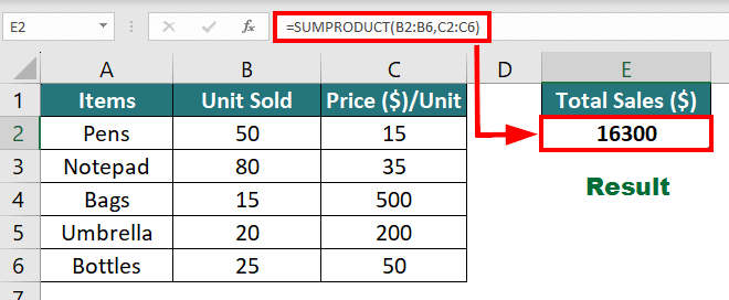
Suppose you need to calculate the overall sales generated by all items. The SUMPRODUCT formula will be as follows:
Result: The formula displays “16300”, i.e., total sales of all the items.
This is how the calculation for =SUMPRODUCT(B2:B6,C2:C6) looks like:
= (50×15)+(80×35)+(15×500)+(20×200)+(25×50)
More advanced applications of the SUMPRODUCT function:
8. SUMIF Function
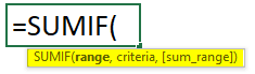
The SUMIF function in Excel adds all the values of a given cell range based on specific criteria.
SUMIF Syntax:
When to use it?
- To calculate the total salary of a specific employee
- Find total sales for a particular quarter
- To determine the total amount you spent on transportation
- Calculate the total marketing expenses of a company, etc.
Example:
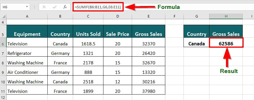
Suppose you have a table with data of a company’s sales in specific countries. You want to find the total gross sales of Canada.
The SUMIF formula will be:
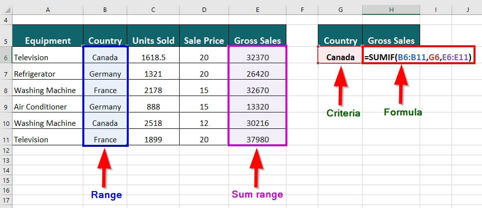
Result: The formula displays “62586”, which is the total gross sales of Canada.
More advanced applications of the SUMIF function:
9. COUNTIF Function
The COUNTIF function in Excel counts the total number of cells in a given range that satisfy a specific condition.
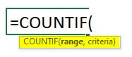
COUNTIF Syntax:
When to use it?
- Counting how many citizens in an area are eligible to vote
- Count the number of students who scored exactly 40 (passing mark)
- Count the total items that are out of stock, etc.
Example:
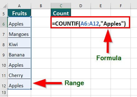
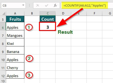
Suppose we want to count the number of apples from a given list of fruits. We can use the below formula:
Result: The formula displays “3”, i.e., a total count of Apples only.
More advanced applications of the COUNTIF function:
10. IF with OR & AND Functions
The IF function in Excel uses logic to decide which value to return. It checks the condition we give and returns a different value depending on whether it is true or false. We can combine the IF function with AND or OR functions as per our requirements.
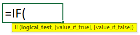
IF Syntax:
When to use it?
IF with OR:
- If the value is Saturday or Sunday, return the day as a weekend else, return it as a weekday
- If it’s a student or a senior citizen, they can redeem discounts, or else they can’t, etc.
IF with AND:
- If the project is on schedule and within budget, display as a project on track, else show the project off track
- A club member can attend a function only if they have a premium membership and donations of more than $5,000, etc.
Example:
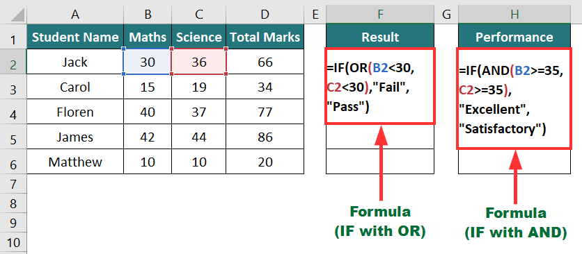
In the data below, we will evaluate students’ results (pass or fail) and performance (satisfactory or excellent) based on certain criteria.
To evaluate the result, we will use IF with OR formula:
To evaluate performance, we will use IF with the AND formula:
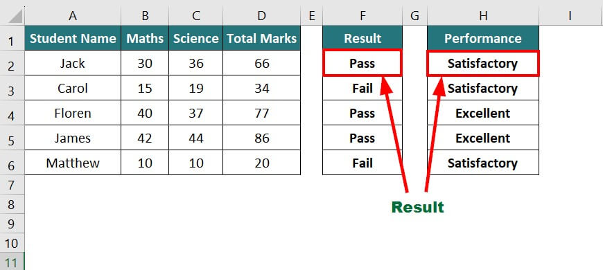
Result: The formula displays “Pass” in the result and “Satisfactory” in performance for student Jack.
More advanced applications of the IF function:
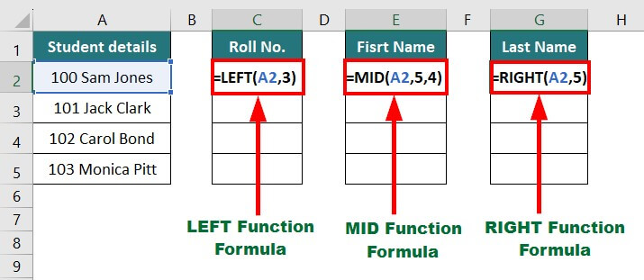
11. LEFT, MID, and RIGHT Functions
The LEFT function in Excel extracts text from the beginning of a given text string (left to right). The RIGHT function extracts text from the right end (right to left). The MID function extracts text from any point in the text string (left to right).
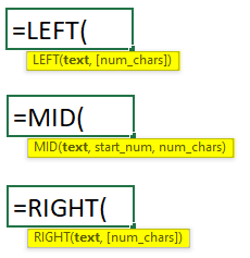
LEFT/ MID/ RIGHT Syntax:
When to use them?
LEFT
- To extract domain names from websites
- To retrieve initials from product code, etc.
MID
- Getting the middle name from a full name.
- To get only the day from the date format MM/DD/YYYY, etc.
RIGHT
- To get the last 4 digits of a person’s social security number
- To know the file extension for any particular file from the file name, etc.
Example:
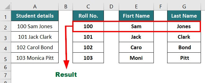
Let’s say you have details of a few students and want to extract their roll no., first name, and last name.
You can use the following formulas:
- To extract roll no.: =LEFT(A2,3)
- To extract the first name: =MID(A2,5,4)
- To extract the last name: =RIGHT(A2,5)
Result: The output of respective formulas are“100”, “Sam”, and “Jones”.
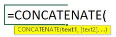
12. CONCATENATE Function
CONCATENATE in Excel is an important function that combines data from different cells and displays the result in a single cell.
CONCATENATE Syntax:
When to use it?
- To combine first name and last name
- To combine pin code and city name for generating address
- To combine domain and page name to create website URL, etc.
Example:
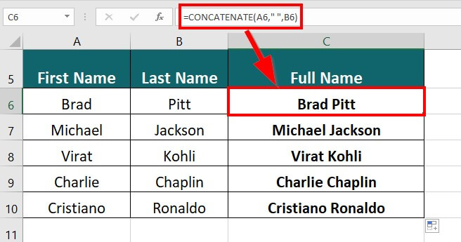
Suppose you have a long list of famous personalities whose first and last names are in different columns, and you want to display their full names in a single column.
The formula for concatenation will be:
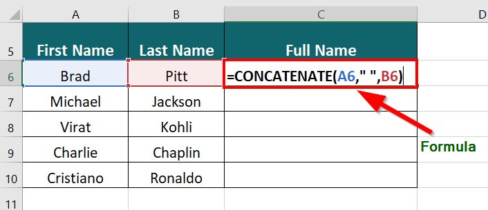
Result: The formula displays “Brad Pitt” in a single column.
13. TRIM Function
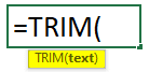
The TRIM function in Excel removes any unwanted or extra spaces from the beginning, in between, or end of a text.
TRIM Syntax:
When to use it?
- To remove extra spaces in between house addresses
- To remove excess spaces in a list of usernames or employee IDs
- To remove leading or trailing spaces from email addresses, etc.
Example:
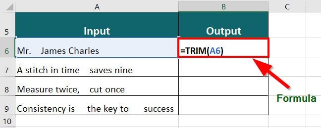
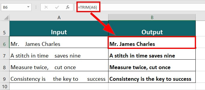
Suppose you have the data below and want to remove any extra space from the sentences.
The TRIM formula will be as follows:
Result: The formula displays “Mr. James Charles” by removing extra spaces.
More advanced applications of the TRIM function:
14. LEN Function
The LEN function in Excel returns the number of characters present in a given text string or data.
LEN Syntax:

When to use it?
- To check the length of a password
- To calculate the number of characters in a pincode
- To check characters of the TIN (Tax Identification Number), etc.
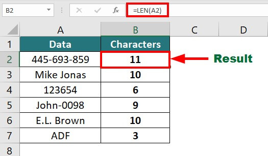
Example:
Suppose you have the below data, and you have to calculate the total number of characters in each cell.
You can use the below formula:
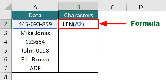
Result: The formula displays 11, i.e., total character in Cell A2.
More advanced applications of the LEN function:
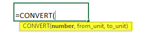
15. CONVERT Function
CONVERT is an advanced Excel formula that converts a number from one measurement unit to another.
CONVERT Syntax:
When to use it?
- To convert temperature from Celsius to Fahrenheit
- To convert minutes to hours or vice-versa
- To convert miles to kilometers or vice-versa
- To convert a liter to a gallon or vice-versa, etc.
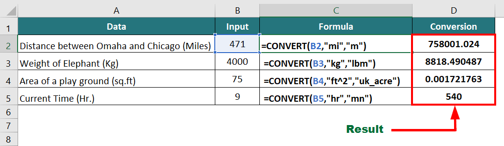
Example:
The below data is in miles, kilograms, square feet, and hours and we need to convert them into meters, pounds, acres, and minutes, respectively,
The formulas will be as follows:
- Miles to meters: =CONVERT(B2,”mi”,”m”)
- Kilograms to pounds: =CONVERT(B3,”kg”,”lbm”)
- Square feet to acres: =CONVERT(B4,”ft^2″,”uk_acre”)
- Hours to minutes: =CONVERT(B5,”hr”,”mn”)
Result: The formula displays the results in the respective cells
16. SORT and SORTBY Functions
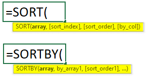
The SORT function is useful to arrange the data in a given array or range in ascending or descending order. On the other hand, the SORTBY function arranges the data of the given array or range based on the sequence or order of another array or range.
SORT and SORTBY Syntax:
When to use them?
SORT Function
- To sort names in alphabetical order
- To arrange product prices in ascending or descending order
- To sort dates from new to old or vice versa, etc.
SORTBY Function
- To sort customers based on their delivery date
- To sort websites based on their ranking
- To sort nations based on population density, etc.
Example:
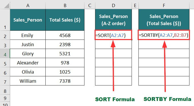
In the below data, in one column, we will organize the salesperson’s name in alphabetical order using the SORT function. Meanwhile, in another column, we will arrange sales person’s names based on their total sales in ascending order using the SORTBY functions. It will show us the best-performing sales employee’s name.
The formulas for both functions will be:
- To sort names in alphabetical order: =SORT(A2:A7)
- To sort total sales in ascending order: =SORTBY(A2:A7,B2:B7)
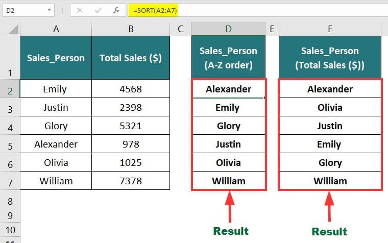
Result: The formula displays the results based on the given condition.
More advanced applications of the SORT and SORTBY functions:
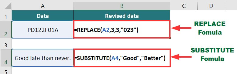
17. REPLACE and SUBSTITUTE Functions
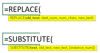
The REPLACE function in Excel replaces a specific number of characters in a given text. On the other hand, the SUBSTITUTE function replaces the entire text string with another text.
REPLACE/SUBSTITUTE Syntax:
When to use them?
REPLACE function
- To replace the year from a date “MM/DD/YYYY” with the new year (replacing 2023 with 2024)
- To replace the extension of a file in the file name
- To replace a particular part of the product code with new data, like PD001 to RP001, etc.
SUBSTITUTE function
- To substitute full form with its abbreviation or acronyms, like “Number” to “No.”
- To substitute errors/incorrect words with correct words, etc.
Example:
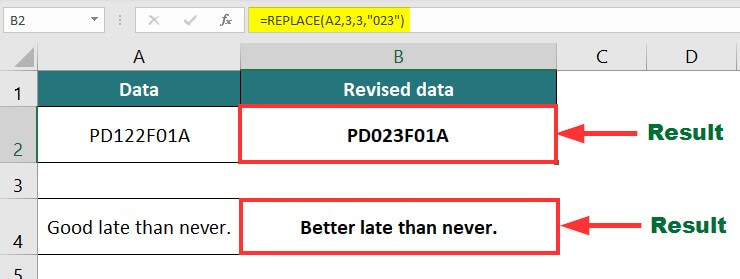
In the below data, we want to replace “122” in Product code PD122F01A with 023 and substitute the word “Good” with “Better” in the phrase.
Formulas for both functions will be:
Result: The output will be as shown in the image below.
More advanced applications of the REPLACE/SUBSTITUTE function:
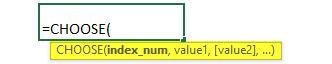
18. CHOOSE Function
You can use the CHOOSE function in Excel to pick a specific value from a list of values by mentioning its position in the list.
CHOOSE Syntax:
When to use it?
- To mention specific calculations based on the command (1= Add, 2= Subtract, 3= Multiply)
- To choose the size of a coffee cup or popcorn box while ordering (1= Small, 2= Medium, 3= Large), etc.
Example:
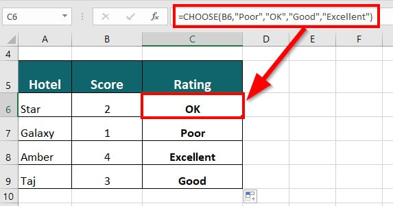
Suppose you want to rate hotels on a score of 1-4, where 1 is Poor, 2 is OK, 3 is Good, and 4 is Excellent.
The CHOOSE function will be as follows:
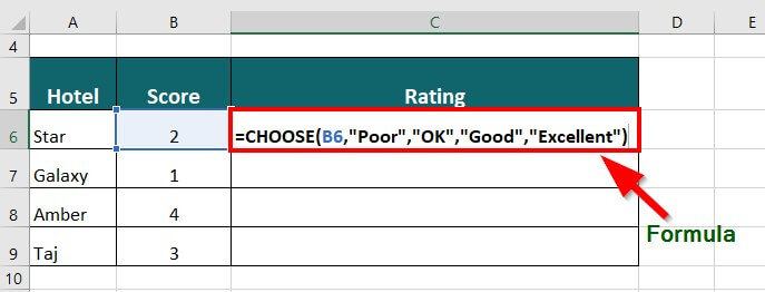
Result: The formula displays “OK” because the score is 2.
19. WORKDAY/NETWORKDAYS
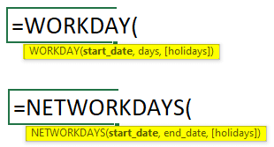
The WORKDAY function in Excel calculates the working date that comes after the mentioned number of working days, starting from the date that we mention. The NETWORKDAYS function returns the number of working days between the start and end date.
WORKDAY/NETWORKS Syntax:
When to use them?
WORKDAY
- Find the deadline date of a project by excluding weekends and holidays
- Calculate the expected date you’ll receive a refund, etc.
NETWORKDAYS
- To calculate the total working days in a month or specific period
- To find the total working days it takes to complete a project, etc.
Example:
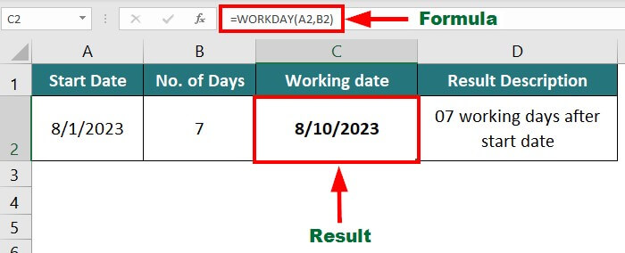
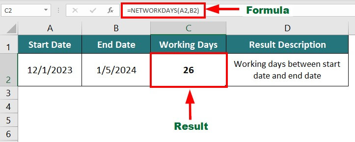
Suppose you want to find the date of the working day after taking a leave of 7 days (excluding holidays) starting from August 1st, 2023. You also want to calculate the number of working days between December 1st, 2023, and January 5th, 2024.
Use the following formula to calculate the work date,
Result: The formula displays “8/10/2023”.
The formula to calculate the no. of working days is as follows:
Result: The formula calculates the working days and displays “26”.
20. PV Function
The PV function is an advanced Excel formula that calculates the present value (PV) of an investment or loan amount. For example, if you want $500 in 3 years at a 10% interest rate, the PV function tells you how much you need to invest today.
PV Syntax:
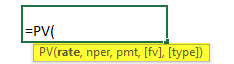
When to use it?
- To know the total money you must save every day to be able to buy a bike in 2 years
- To calculate the amount you need to invest today to be a millionaire in 20 years
- To decide how much you should pay in today’s time to repay your loan in one year, etc.
Example:
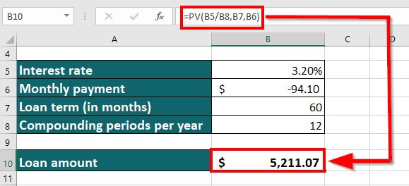
Suppose you know the interest rate, monthly payment, loan term, and compounding period and want to calculate the loan amount.
You can input the values as follows:
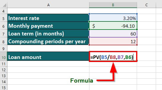
Result: The formula displays the result as “$5,211.07”.
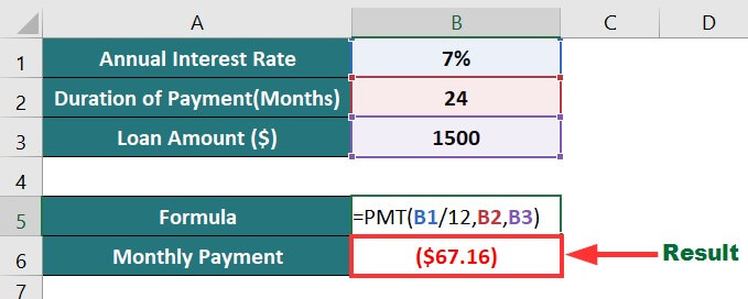
21. PMT Function
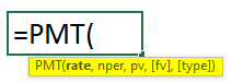
Excel’s PMT (PAYMENT) function calculates the monthly or periodic payment for a loan based on the interest rate, duration, and loan amount.
PMT Syntax:
When to use it?
- To estimate the monthly payment for a loan
- To estimate regular installment for a credit card debt
- To calculate periodic premiums for an insurance policy scheme, etc.
Example:
We want to calculate the monthly payment of a loan of $1500 for 24 months with an annual interest rate of 7%.
The formula for calculating the monthly payment will be:
Result: The formula’s output is “$67.16” (monthly payment).
More advanced applications of the PMT function:
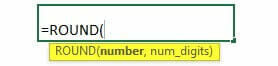
22. ROUND Function
The ROUND function in Excel lets us decide if we want a numerical value to have any decimal points or not, and if yes, how many decimal places the number should have.
ROUND Syntax:
When to use it?
- To round off a student’s scores to a whole number (rounding 90.8% to 91%)
- Round off the temperature to a whole number (rounding 23.8°C to 24°C)
- To round off a currency exchange rate to a certain decimal place (rounding 0.7856 to 0.79), etc.
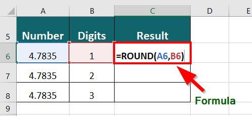
Example:
In the below data, you have to round the given decimals numbers to one, two, and three decimal places, respectively.
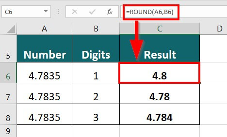
The formula for the ROUND() function will be:
Result: The formula displays “4.8” with one decimal point.
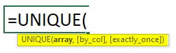
23. UNIQUE Function
The UNIQUE function in Excel returns a list of unique values in a given range.
UNIQUE Syntax:
When to use it?
- To find a unique product category from a product list
- To obtain a list of cities from customer addresses
- To extract invoice or bill numbers from a financial report
- To get a unique employee_Id from the employee database, etc.
Example:
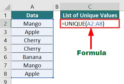
Here, we need to find the unique values in the table below, which has various fruits’ names.
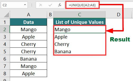
Use the below formula for the UNIQUE() function:
Result: The formula displays the unique values from the given array.
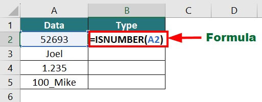
24. ISNUMBER Function
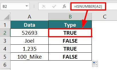
The ISNUMBER function checks if a cell value is in text or numeric form. It returns TRUE for numeric value and FALSE for text value.
ISNUMBER Syntax:

When to use it?
- To check if the cell is in number format before performing mathematical calculations
- To check if a cell has a valid currency value
- Check the format of cells with #DIV/0! or #VALUE! Errors, etc.
Example:
In the data below, we will determine whether values entered in a cell are in numeric or text form.
Enter the below formula in the respective cell,
Result: The formula “TRUE” for numeric values.
25. Goal Seek
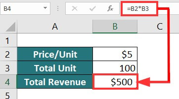
As the name suggests, Goal Seek is an in-built advanced Excel tool that helps us find the specific value that we need to reach the mentioned value (our goal).
When to use it?
- To calculate how many units of a product we must sell to reach the target profit
- To find the minimum products you must produce to meet public demand
- Check where we can cut expenses to achieve the cost savings target, etc.
Example:
If you sell 100 units for $5 each, your total revenue will be $500. Now, you want to figure out how many units you must sell to make a total revenue of $1255.
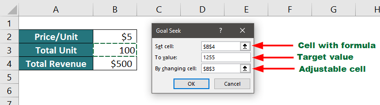
Let’s see how to use Goal Seek to accomplish this task.
- Go to the “Data” tab, click “What-If-Analysis” under the Forecast group, and select “Goal Seek”.
- Enter the target value and choose the desired cell, as shown below.
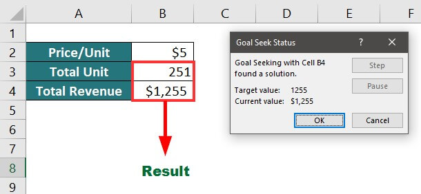
Result: The output is “$10”.
It means you must sell 251 units at $5 to make a total revenue of $1255.
More advanced applications of the Goal Seek function:
These were the 25 most advanced functions and formulas of Excel. Now, let’s see a case study where we will use some of these functions to create a travel planner.
Case Study – Switzerland Travel Planner

Emily loves traveling, and she is planning a trip to Switzerland. For that, she uses advanced Excel functions to make a budget, track her expenses, convert currency, and much more.
Let’s see how she uses different functions for planning her trip. You can download Emily’s travel planner to understand better.
1) Currency Conversion (VLOOKUP Function)
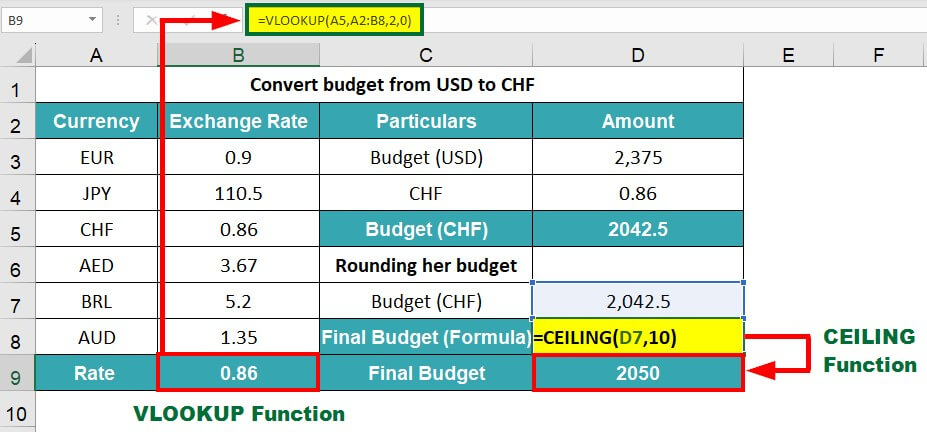
First, Emily uses the VLOOKUP function to find the exchange rate for converting USD to CHF. She then converts her budget of $2,375 into Swiss Franc (CHF). After that, she rounds off the converted budget to the nearest 10 using the CEILING function.
2) Choose Trip Dates (WORKDAY Function)
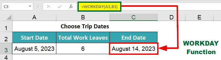
Emily has six paid leaves pending, which she wants to use for this trip. She uses the WORKDAY function to find the length of her trip. This function considers the start date and trip duration and excludes weekends and holidays to calculate the end date. Using this function, Emily can plan a trip for 10 days, using all 6 of her leaves and four weekend dates.
3) Make an Itinerary (CONCATENATE Function)
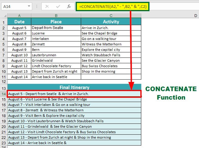
She first makes a detailed table of all the places she wants to visit, along with the corresponding activities and dates. Then, she uses the CONCATENATE function to create a comprehensive itinerary by combining the date, place, and activity.
4) Calculate Expenses (SUMIF Function)
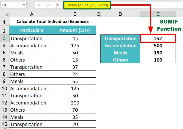
After returning, Emily wants to check how much she spent on each aspect of the trip: accommodation, meals, transportation, and others. She added the expenses for all these items to her expense list every 2-3 days. Using her list of all her expenses, she uses the SUMIF function to calculate the total money spent for each type of expense.
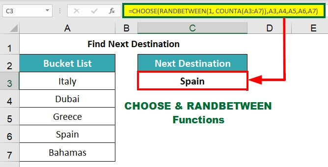
5) Find the Next Destination (CHOOSE & RANDBETWEEN Functions)
Finally, Emily wants to decide her next trip destination, for which she uses the CHOOSE and RANDBETWEEN functions to select her next destination from a list of destinations randomly.
Conclusion
We can see how Emily’s proficiency in using advanced Excel formulas and functions helps her very easily plan a detailed trip to her favorite destination, keeping her work, expenses, and interests in mind. By using SUMIF, WORKDAY, CONCATENATION, VLOOKUP, and CHOOSE, she effectively tracks expenses, manages her itinerary, and analyzes her travel spending. Similarly, you can use other advanced Excel functions to make your travel planner or for any other purposes.
Frequently Asked Questions(FAQs)
Q1. What are the top 10 Excel formulas?
Answer: The top 10 Excel formulas are:
- VLOOKUP Function
- XLOOKUP Function
- IFERROR Function
- INDEX Function
- MATCH Function
- OFFSET Function
- SUMPRODUCT Function
- SUMIF Function
- COUNTIF Function
- IF combined with AND/OR Functions
Q2. What is the importance of studying advanced spreadsheet skills?
Answer: Once you become skilled in using advanced Excel formulas and functions and various tools, you can easily solve a wide range of real-world math problems. Knowing advanced spreadsheet skills helps you arrange your data however you want, create tables, graphs, charts, etc., perform all calculations in a second, and so much more. It doesn’t matter what field you work in; learning advanced Excel formulas and functions can definitely benefit you.
Q3. What are the advanced Excel skills for accountants?
Answer: The Advanced Excel skills that would be helpful for accountants are:
1. Vlookup to find data from an extensive database
Example: Using Vlookup to match the payment amount for a particular receipt number with the payment amount in the invoice bills.
2. Pivot tables to prepare reports
Example: Using pivot tables to create an annual budget report by combining and analyzing data of incoming and outgoing cash.
3. Data Validation to create drop-down lists
Example: Making a drop-down list of all expenses included in a business trip.
4. Using Proper Cell Referencing
Example: Building a template using cell referencing that automatically updates the new values whenever new data is added to any sheet.
5. Logical Analysis using IF, AND, and OR functions
Example: Using the IF AND function to automatically check if the credit and debit sides match in each journal entry.
Recommended Articles
This article has provided the 25 advanced Excel formulas and functions used in business. You can also check out the below articles to learn other applications of advanced Excel formulas and functions
