Updated July 1, 2023
Introduction to Goal Seek in Excel
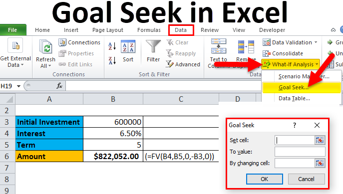
Goal Seek is a tool in Microsoft Excel for finding out an unknown value from a set of known values. This simply means that it helps you find the missing number when you know some of the numbers involved in a calculation.
For example, if you want to know how much money you should save annually for retirement, but do not know the interest rate, Goal Seek can help you find the interest rate needed to reach your goal.
Goal Seek is a powerful tool for performing What-If analysis and can have a wide range of applications, such as finance and engineering. In finance, it’s especially useful for financial models, budgeting, and forecasting.
How to Implement Goal Seek?
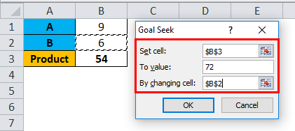
Goal Seek is implemented using the Goal Seek dialog box, as shown in the following figure:
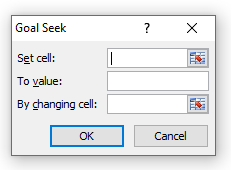
One can see that the Goal Seek dialog box accepts three values:
- Set Cell: The “Set Cell” refers to the specific cell in your worksheet that needs to be changed to achieve the desired outcome.
- To Value: The “To Value” is the intended value that you want the “Set Cell” to be changed to.
- By Changing Cell: This is the cell in your worksheet that will be changed by Excel’s Goal Seek tool in order to achieve the “To Value” for the “Set Cell”.
How to Use Goal Seek in Excel?
Goal Seek in Excel is very simple and easy to create. Let’s understand the working with some examples.
Example #1
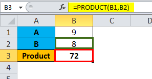
Let’s consider a simple example of multiplying two numbers, A and B. In this example, A has a value of 9, while B has a value of 6.
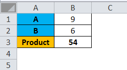
To find the product of these two numbers, we can use the function =PRODUCT(B1,B2), which results in 54.
Now, let’s say we want to find out the value of B, if value of A is still 9, and the desired product is 72.
To do this, we can use Excel’s Goal Seek tool.
Solution:
The following are the steps for calculating it:
- Click on the “Data” tab
- Under the Data Tools group, click on the “What-If Analysis” drop-down menu
- Click on “Goal Seek”
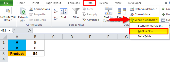
- The user will see the “Goal Seek Dialog Box” appear on their screen.
- Within this dialog box, the user must navigate to the “Set cell” field and select “B3“.
- In the “To value” field, the user must input the value “72“.
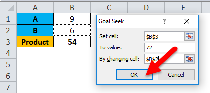
- Next, the user must navigate to the “By changing cell” field and select “B2“
- Then proceed to click on “OK”.
The result is as follows:
Example #2
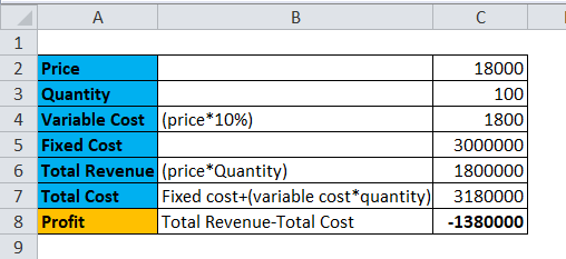
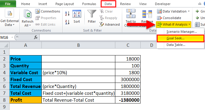
Aryan Ltd. operates in the generator business and sells each generator at a price of Rs. 18000 and the quantity sold is 100.
One can observe in the below table that the company is suffering a loss of Rs. 13.8 lacs. Furthermore, the maximum price for which a generator can be sold is identified to be Rs. 18000. Now, one must identify the no. of generators that can be sold, which will return the break-even value (No Profit No Loss). Thus, the Profit value (Revenue – Fixed Cost + Variable cost) needs to be zero in order to attain a break-even value.
Solution:
The calculation includes the following steps:
- Click on the “Data” tab
- Under the Data Tools group, click on the “What-If Analysis” drop-down menu
- Click on the “Goal Seek” option
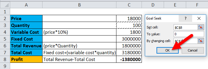
- Within the “Goal Seek” dialog box, the user should then select “C8” in the “Set Cell” field.
- Next, the user should enter the value “0” in the “To Value” field.
- Finally, the user should select “C3” in the “By Changing Cell” field.
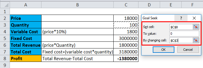
- Then proceed to click on the “OK”
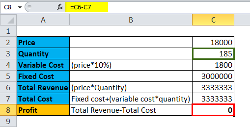
The result is as follows:
Example #3
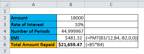
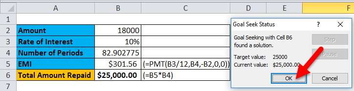
In the given scenario, a man has borrowed a loan amount of Rs. 18,000 with an interest rate of 10% per annum. This results in a monthly repayment of Rs. 481.32 and a total repayment amount of Rs. 21659.47 after the completion of the loan term, which is 45 months.
However, the borrower has found it difficult to pay the current monthly amount and wishes to extend the repayment period. At the same time, the borrower wants to ensure that the total repayment amount does not exceed Rs. 25000.
Let’s resolve this using Goal Seek:
Solution:
The calculation includes the following steps:
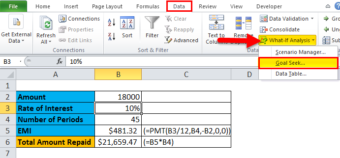
- Click on the “Data” tab
- Under the Data Tools group, click on the “What-If Analysis” drop-down menu
- Click on the “Goal Seek” option
- In the Goal Seek Dialog Box, the borrower must select cell “B6” in the “Set Cell” field.
- Next, the borrower must enter the value of “ 25000” in the “To Value” field.
- Finally, the borrower must select cell “B4” in the “By Changing Cell” field.
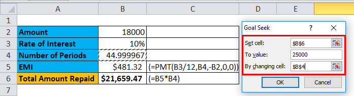
- Click on the “OK” button to initiate the calculation.
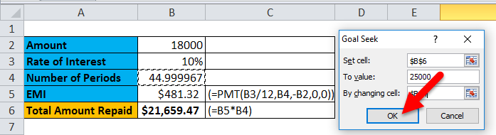
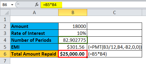
- Goal Seek lowers the monthly payment, and the number of payments in cell B4 changes from 45 to 82.90. As a result, the Equated Monthly Instalment (EMI) is decreased to 301.56.
- Press the “OK” button to accept the changes made by Goal Seek.
The result is as follows:
Example #4
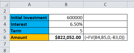
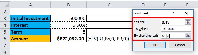
In the above table, a man is considering investing a lump sum amount in his bank for a specific time period. The bank employee recommends opening a Fixed Deposit Account with an interest rate of 6.5% and a term of 5 years. To calculate the return, the man uses the FV function, as demonstrated in the calculation procedure given above.
Now, the man desires to increase his return to $1500000 without altering the time period or initial amount of investment. Therefore, he wishes to determine the interest rate that will enable him to achieve the desired return.
The calculation includes the following steps:
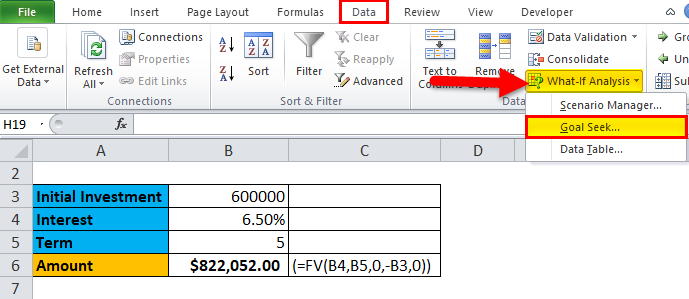
- Click on the “Data” tab
- Under the Data Tools group, click on the “What-If Analysis” drop-down menu
- Click on the “Goal Seek” option
- Open the Goal Seek Dialog Box and select “B6” in the “Set Cell” field.
- Enter “1500000” in the “To Value” field.
- Select “B4” in the “By Changing Cell” field to change the rate of interest.
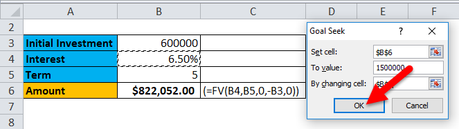
- Click on “OK” to proceed.
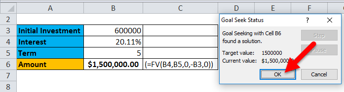
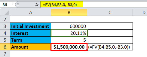
- Goal Seek adjusts the interest rate in cell B4 from 6.50% to 20.11%, while keeping the initial investment and number of years unchanged.
- Press OK to accept the changes made by the Goal Seek function.
The result is as follows:
Real-World Examples
1. Finance
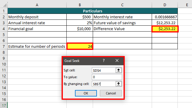
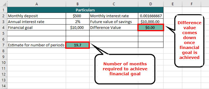
Suppose you are aiming to save $10,000 as a down payment for a house and intend to make regular monthly deposits into a savings account with a 2% annual interest rate. You want to calculate the number of months it will take to reach your objective.
2. Marketing
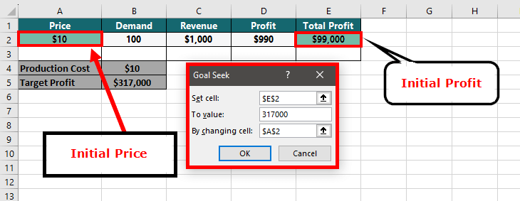
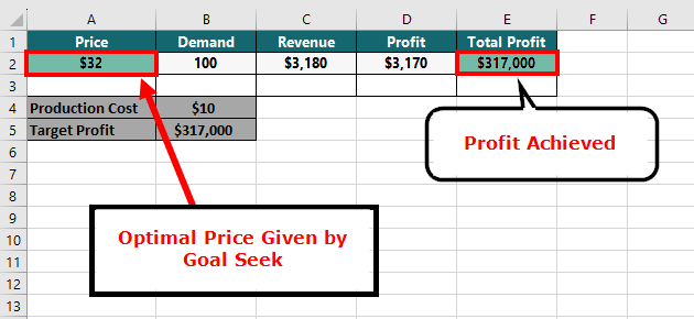
Suppose you are a marketer who wants to determine the optimal pricing strategy for a product. You have data on the production cost of the product and on its demand and revenue at different price points. You can use Goal Seek to find the price that will maximize the revenue while considering the production cost of the product. For example, Goal Seek can help find the price point that will give the maximum profit for a product with a certain production cost and demand.
3. Operations
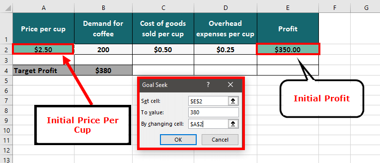
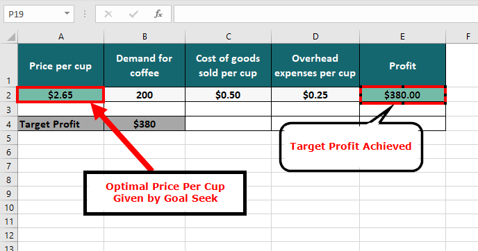
Suppose you are the manager of a coffee shop and want to determine the optimal price to charge for a cup of coffee. You have data on the cost of goods sold, overhead expenses, and the demand for coffee at different price points.
Pros & Cons of Goal Seek in Excel
- Goal Seek allows the user to find accurate data by back-calculating the resulting cell by giving a specific value to it.
- Goal Seek can work with the Scenario Manager feature as well.
- Data must contain a formula to work.
Things to Remember
- Goal Seek can only handle one input and one output cell. It cannot handle multiple constraints.
- Goal Seek may fail to find a solution when the input value is far from the desired output value.
- Since Goal Seek is dependent on initial input values, it can lead to suboptimal solutions if the initial input value is too far from the optimal value.
- Goal Seek may not be suitable for complex models, which have many input and output cells. Instead, one can use other Excel tools such as Solver or Visual Basic for Applications (VBA).
- The model must be set up correctly before using Goal Seek, ensuring that all cells are properly formatted and excluding any circular references.
- When using Goal Seek, it is recommended to use cell references instead of hard-coding values for easy changes in the future.
- Goal Seek can work with other Excel functions, like data tables, scenarios, or macros to automate multiple calculations.
- Make a backup copy of the file before using Goal Seek, especially if significant changes are being made to the model.
- Always consider your model’s real-world applications and Goal Seek’s limitations when deciding which tool to use.
Frequently Asked Questions
Q1. What are some common applications of Goal Seek in Excel?
Answer: There are various applications of Goal Seek in Excel, such as:
- Calculating the required monthly payment to pay off a loan in a certain time
- Calculating a suitable price for a product that can maximize profits
- Determining the break-even point in sales volume for a business
- Finding the necessary discount rate to achieve a desired net present value for a project
- Determining the optimal production volume to minimize costs and maximize profits.
Q2. What is the primary difference between Goal Seek and Solver in Excel?
Answer: Goal Seek is a simpler tool used for finding a single input value that will result in a specific output value that allows, Solver is a more powerful tool that can handle more complex problems with multiple constraints and variables.
Q3. What are the limitations of Goal Seek in Excel?
Answer: There are multiple limitations to Goal Seek in Excel, such as that it works with only one variable, is restricted to linear relationships, finds only a single solution, etc. Hence, Goal Seek is not suitable for complex problems.
Recommended Articles
This is our guide to Goal Seek in Excel. Here are some further articles for expanding understanding:
