Updated May 9, 2023
SUMIF with Multiple Criteria (Table of Contents)
- Excel SUMIF Function with Multiple Criteria
- How to Use SUMIF Function with Multiple Criteria in Excel?
Excel SUMIF Function with Multiple Criteria
SUMIF in Excel is used for calculating the total of any specified criteria and range, unlike the sum function, which is a single shot that calculates the total of the whole range without any specific criteria. We can use SUMIF for adding or subtracting different criteria ranges.
It can be accessed from Insert Function from the Math & Trig category.
Syntax for SUMIF
For better understanding, we have shown the syntax below.
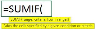
Arguments of SUMIF Function:
- Range – This first range is the range we need to calculate the sum.
- Criteria – It is for fixing the criteria for what part of the range we need to calculate the sum.
- Sum_Range – That range needs to be summed for defined criteria.
How to Use Excel SUMIF Function with Multiple Criteria?
Let’s understand how to use Multiple Criteria using examples in Excel.
Examples of SUMIF with Multiple Criteria
Example #1
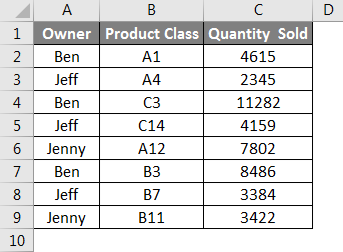
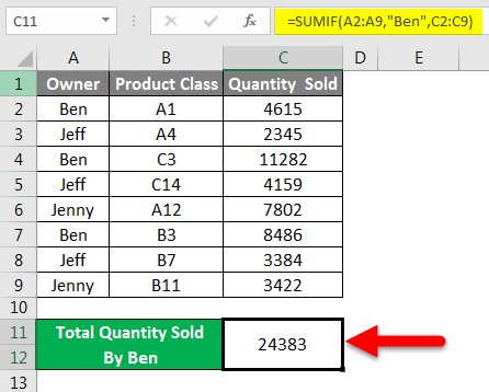
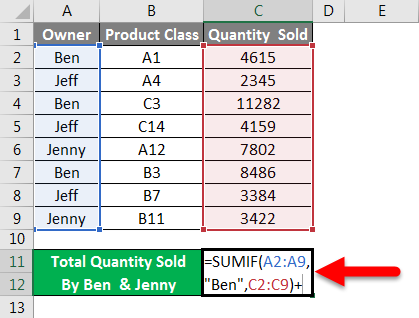
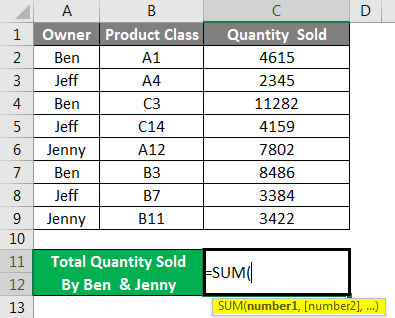
We got the sales data for some product class. As we can see below, the data we have has the owners’ names and the quantity sold by them for the respective product class.
Now we will apply multiple criteria in the simple SUMIF function.
Considering the multiple criteria for calculating the sum of the above-shown data, we need to apply SUMIF to get the sum of more than 1 owner’s quantity sold data. Here we will calculate the total quantities sold by Ben and Jenny together.
For this, go to the cell where we need to see the output and type the “=” (Equal) sign. This will enable all the inbuilt functions of Excel. Now search and select the SUMIF function from the search list.
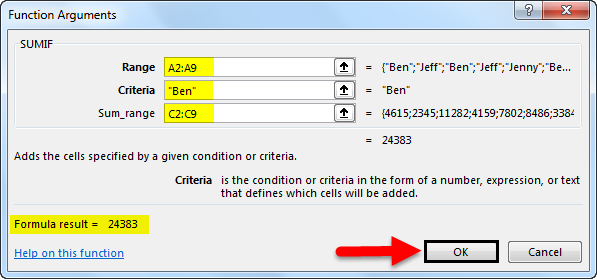
For calculating the sum of quantities sold by Ben, select the Owner’s name as in range, criteria as BEN, and sum range as complete Quantity Sold column C and press enter.
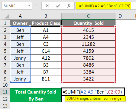
We will get the sum of Ben’s sold quantity as 24383.
To add another criterion in this syntax, we will add the quantity sold by Jenny with the help of the “+” sign, as shown below.
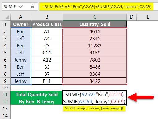
Now press enter to get the total sum.
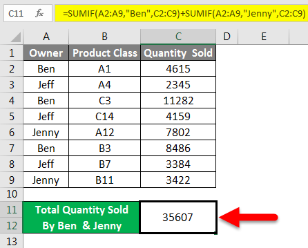
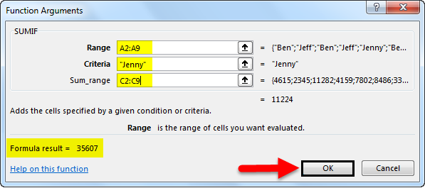
As we can see in the above screenshot, the quantity sold by Ben and Jenny together is coming to 35607. We can cross-check the sum separately to match the count with the SUMIF function.
Example #2
There is another way to apply SUMIF criteria. For this, go to the cell where we need to see the output and click on the Insert function besides the formula bar, as shown below.
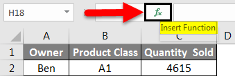
We will get the Insert Function window. Select the function SUMIF or an ALL category from there, as shown below.
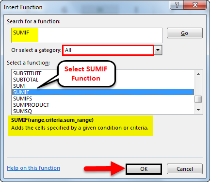
We can see the suggested syntax at the bottom of the window. And click on, Ok.
In the functional argument box, select the A2 to A9, Criteria as Ben, and sum range from C2 to C9 and click Ok. This will frame the first half of the multiple criteria syntax.
Now insert plus sign (+) as shown below.
And click on Insert Function and search for SUMIF and click on Ok, as shown below.
And now, in the second half of the arguments of SUMIF, multiple criteria select the range and sum range same as selected for the first half of the syntax and enter criteria as Jenny. Once done, click on, Ok.
If we see the complete syntax, it will look like as shown below.
Now press enter to see the final output.
As we can see in the above screenshot, the output of SUMIF with multiple criteria is 35607, as we got in example 1.
Example #3
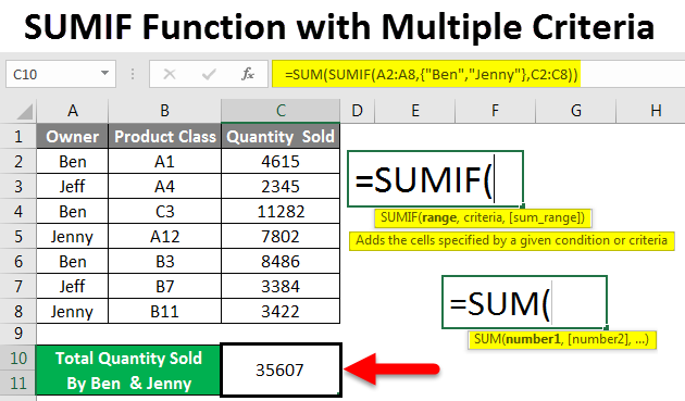
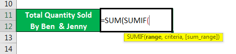
There is another method of using SUMIF with multiple criteria. Here we will use the same data which we have seen in example-1. We will also86+ see the calculated value of quantity sold by Ben and Jenny to compare the result obtained from this method with the result in example-1.
We will use Sum with SUMIF with multiple criteria of Ben and Jenny’s quantity sold.
Now go to the cell where we need to see the output of SUMIF and type the “=” sign, and search and select the Sum function first.
Now search and select the SUMIF function as shown below.
Select the range as A2 to A9, set the criteria as Ben and Jenny in inverted commas under curly brackets { }, and select the sum range as C2 to C9, as shown below.
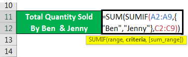
Note: Adding Criteria in curly brackets is necessary. This allows the multiple criteria in the formula. Now press enter to see the result, as shown below.
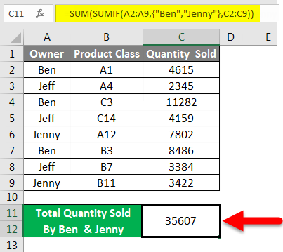
As we can see, the calculated result in example-1 and example-2 are equal. Which says our use of multiple criteria for this example is also correct.
Pros and Cons of SUMIF with Multiple Criteria
Pros
- It is good to use multiple criteria with SUMIF to get the result quickly.
- The syntax may look complex, but using it once is better than using it in different cells and later adding it up.
- We can insert as many criteria as required.
Cons
- As the syntax for multiple criteria, SUMIF has more than 1 criterion, so sometimes it becomes complex to rectify the error.
Things to Remember
- Use curly brackets {} if you use SUMIF with multiple criteria, as shown in example-3. And in that curly brackets, enter the content manually instead of framing it with cell selection. Curly brackets support only text entered in them.
- Syntax of example 3, i.e., calculating sum with multiple criteria, is small and easy to use, so it is always recommended.
Recommended Articles
This is a guide to SUMIF Function with Multiple Criteria in Excel. We discuss using SUMIF Function with Multiple Criteria, practical examples, and a downloadable Excel template here. You can also go through our other suggested articles –
