Introduction to INDEX MATCH Function
Being an Excel user, we often rely on VLOOKUP, in the worst-case HLOOKUP formula, to look up the values inside a given range of cells. However, it is a well-known fact that VLOOKUP has its own limitations.
For example, we can’t look up the values from right to left if you are using VLOOKUP as a function, and this is where I believe users across the globe might have started to find out an alternative for this function. As far as an alternative is concerned, there is an alternative to VLOOKUP, which is more versatile and called INDEX MATCH popularly. In this article, we will see how INDEX MATCH Function in Excel works with the help of some examples.
The syntax for INDEX MATCH
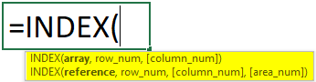
As said earlier, INDEX and MATCH combine to lookup the value in a given range. It has the syntax below:
Arguments:
INDEX() – Formula that allows you to capture the value from a given cell through the table associated with a column or row number.
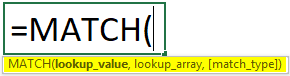
MATCH() – The formula matches the lookup value in a given array and provides its position as an argument to the INDEX function.
How to Use the INDEX MATCH Function in Excel?
Through this example, we will see how INDEX MATCH can be used as an alternative to VLOOKUP.
Example #1 INDEX MATCH as an Alternative to VLOOKUP
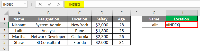
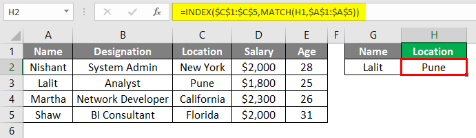
Suppose we have data as shown in the screenshot below:
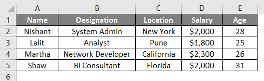
We will capture the Location column with the Name column as a reference (for the name Lalit).
Step 1: In cell H2, start typing =INDEX and double click to select the INDEX formula from the list of all possible functions starting with the keyword INDEX.
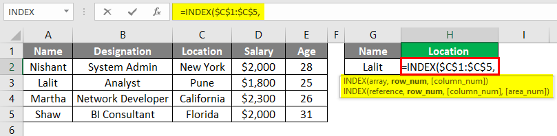
Step 2: Use $C$1:$C$5 (Location column) as an argument to the INDEX formula (this is an array from where we want to pull the lookup value for a match). The dollar sign emphasizes that the range C1:C5 is made constant for the processing of this formula.
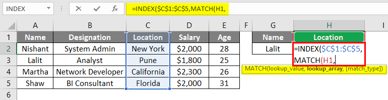
Step 3: Use the MATCH formula as a second argument inside the INDEX formula and use a value in H1 as a lookup value under the MATCH formula.
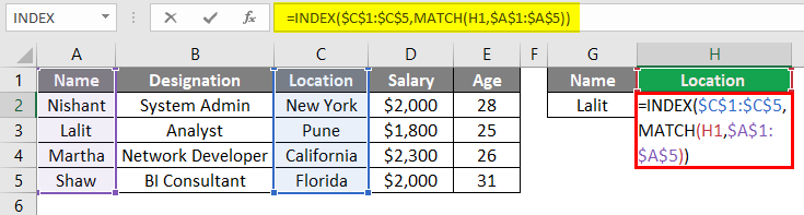
Step 4: Select the lookup array from A1:A5, as this is the column where we want to check whether the lookup value can be found. Also, use zero as an exact match argument inside the MATCH function, as zero looks up for the exact match of the lookup value.
Step 5: Close the parentheses to complete the formula and press Enter key to see the output. We could see the Location as Pune, which is looked up based on the lookup value Lalit.
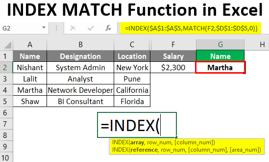
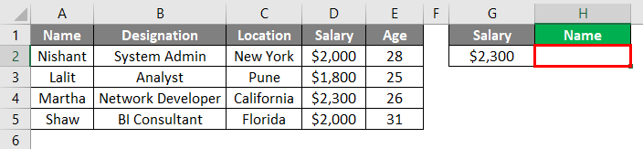
Example #2 INDEX MATCH for LOOKUP from Right to Left
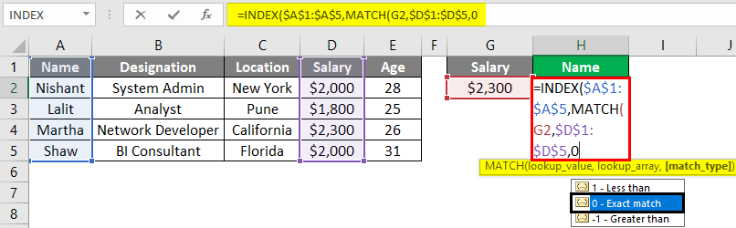
Suppose a scenario where we have a salary as a lookup value, and we need to figure out with whom that salary is associated.
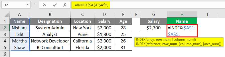
Step 1: Start the formula with =INDEX and use A1:A5 as an array argument under cell H2 of the current worksheet.
Step 2: Use the MATCH formula under INDEX as a second argument. Inside MATCH, use H1 as a lookup value argument.
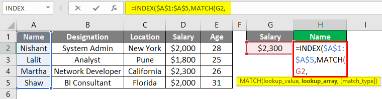
Step 3: D1:D5 would be your lookup array. The formula will search the lookup value in this array and give the position of the same as an argument to the INDEX formula. Don’t forget to use zero as a matching argument.
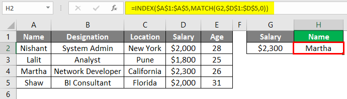
Step 4: Close the parentheses to complete the formula and press Enter key to see the output. You can see the name Martha in H2 and can verify that she is the one who has a salary of $2,300.
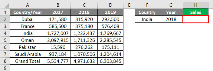
Example #3 INDEX MATCH to LOOKUP Values from Rows and Columns
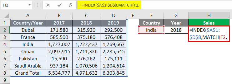
Suppose we have data as shown below, and we need to look up sales value for India in 2018. We need to do two types of matching, one for the Country and another for the Year. See how it goes with INDEX MATCH.
Step 1: Input =INDEX formula and select all the data as a reference array for the index function (A1:D8).
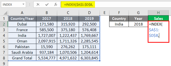
We need to use two MATCH functions to match the country name and the other matching the year value.
Step 2: Use MATCH as an argument under INDEX and set F2 as a lookup value. This is the MATCH for COUNTRY.
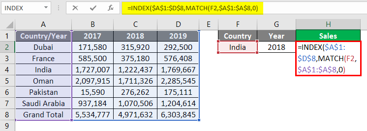
Step 3: Use A1:A8 as a lookup array to find the specified country name. Don’t forget to use zero as a matching criterion that specifies an exact match.
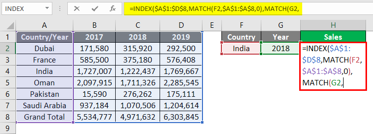
Step 4: Now, again, use the MATCH function, which allows the system to check 2018 and assign the position of Sales value associated with India to the INDEX formula. Set the lookup value as G2 inside the MATCH formula.
Step 5: Here, we could see only cells A1:D1, where we could find the lookup value 2018. Thus, use the same as a lookup array for the MATCH formula.
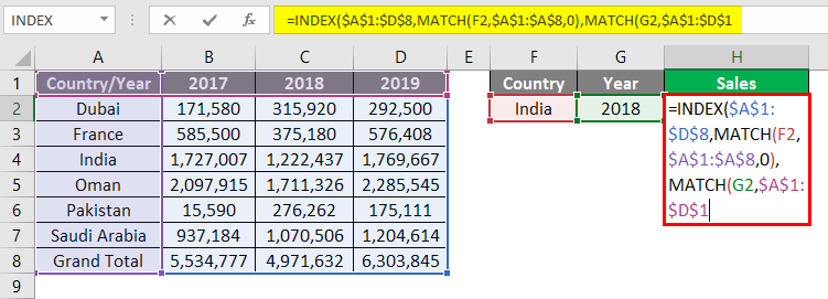
Step 6: Use zero as matching criteria that specify the exact match for the year value inside the lookup range. Close the parentheses and press Enter key to see the output.
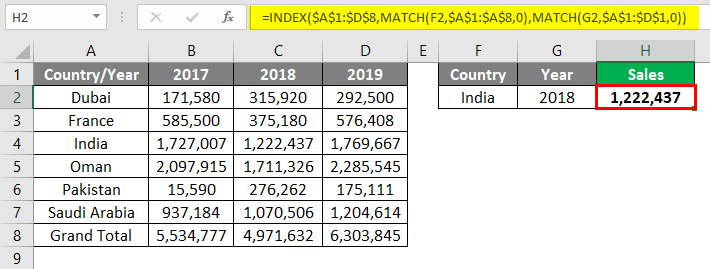
We can see that the function has captured the correct value for the 2018 sales value associated with India. This is how we can use the INDEX MATCH function under different scenarios. Let’s wrap things up with some points to be remembered.
Conclusion
INDEX MATCH is not a function in Excel; rather, it is a combination of two different formulae and is more powerful than VLOOKUP (we will check this in short). This function can be used on rows, columns, or a combination of both, making it a successor of old-school VLOOKUP, which can only work on columns (vertical lines). This combination is so relevant that some analysts even prefer to look up the values and never move their heads towards VLOOKUP.
Things to Remember
- INDEX MATCH is not a function in Excel, but a combination of two formulas, INDEX, and MATCH
- INDEX MATCH can be used as an alternative to old-school VLOOKUP. VLOOKUP only can see through the vertical cells. In contrast, INDEX MATCH can look up values based on rows, columns, and a combination of both (see example 3 for reference).
Recommended Articles
This is a guide to the Index Match function in Excel. Here we discuss how to use the Index Match function in Excel, practical examples, and a downloadable Excel template. You can also go through our other suggested articles –
