Updated August 21, 2023
SUMPRODUCT Function with Multiple Criteria (Table of Contents)
SUMPRODUCT Function with Multiple Criteria
Sumproduct in Excel calculates the multiplication of 2 numbers and then adds all the multiplied numbers in one go. To use Sumproduct multiple criteria, we can use different conditions for a single source of data, such as for the addition of multiplied number, we can feed the condition on which we want Sumproduct. For example, applying sumproduct in student’s data with multiple criteria, we can choose the student names or class as criteria to apply Sumproduct.
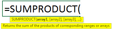
The syntax for SUMPRODUCT:
Parameters:
- array1:-Which denotes the first array or range that we need to multiply, and then it will add the value subsequently.
- array2:- This denotes the second array or range that we need to multiply, and then it will add the value subsequently.
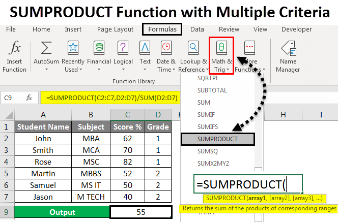
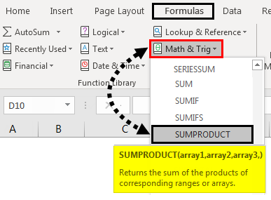
SUMPRODUCT function normally multiplies the ranges or arrays together and then returns the sum of products. This “SUMPRODUCT” is a versatile function where it can be used to count and sum like COUNT IFS and SUMIFS functions. We can find the SUMPRODUCT built-in function in Excel, categorized under the MATH/TRIG function, where we can find it in the formula menu, shown in the below screenshot.
How to use SUMPRODUCT Function with Multiple Criteria?
Let’s use some examples to understand how to use SUMPRODUCT Function with Multiple Criteria.
Example #1
In this example, we will learn how to use the SUMPRODUCT function using simple arithmetic values.
Consider the example below, which has some random numbers in two columns shown below.
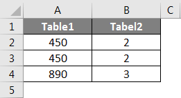
We must multiply the A and B column values and sum the result. We can do it by applying the SUMPRODUCT function following the steps below.
Step 1 – Click on the cell where you want the result.
Step 2 – Apply the SUMPROODUCT formula as shown below.
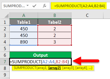
In the above screenshot, we have applied the SUMPRODUT function with A2:A4 as array1 and B2:B4 as array two, which will multiply both the values and sum the result.
Step 3 – Click the Enter key to get the final output, as shown below.
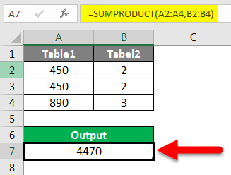
Result:
In the below screenshot, we can see that SUMPRODUCT has returned the output of 4470. Where this SUMPRODUCT function calculates the array as =(450*2)+(450*2)+(890*3)=4470
Example #2 – Using Multiple SUMPRODUCT
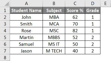
In this example, we will see how to use the multiple SUMPRODUCT functions by using student’s marks scored in the semester, as shown below.
Consider the above example where we need to multiply both A and B column values and calculate the average by following the below steps.
Step 1 – Create a new column for output.
Step 2 – Apply the SUMPRODUCT function =SUMPRODUCT(C2:C7,D2:D7)/SUM(D2:D7) which is shown below.
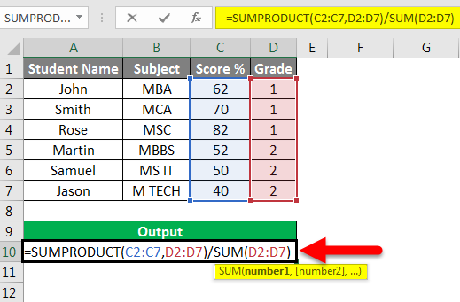
Step 3 – Click the Enter key to get the average result percentage of 55 %, shown in the screenshot below.
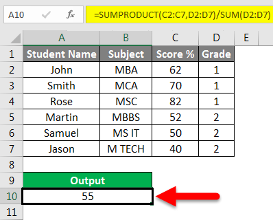
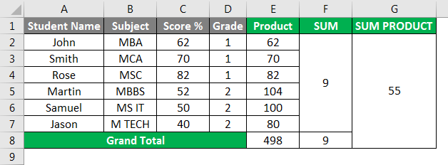
In the above screenshot, we applied the SUMPRODUCT function with the first array as score values C2 to C7 and the second array as Grade Value D2 to D7 so that we sum-product will multiply the values first where if we do a manual calculation, we will get the product value as 498 and the sum value as 9 and divide the Product value by sum value which will give you the same result as 55 percent which is shown as the manual calculation in the below screenshot.
Manual Calculation:
Example #3 – Using TRUE & FALSE in SUMPRODUCT with Criteria
This example will teach us how to apply SUMPRODUCT to get specific criteria-based data.
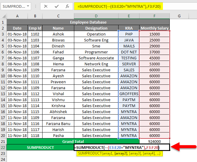
Consider the below example, which shows the employee database with their EmpID, Name, Designation, KRA, and Monthly Salary.

We need to check how many employees work in a specific “KRA” and their grand total salary. In such cases, we can easily calculate the output by applying the SUMPRODUCT function by following the below steps.
- Create a new row for the output column.
- Apply the below SUMPRODUCT function as follows.
=SUMPRODUCT(–(E3:F20=”MYNTRA”),F3:F20)
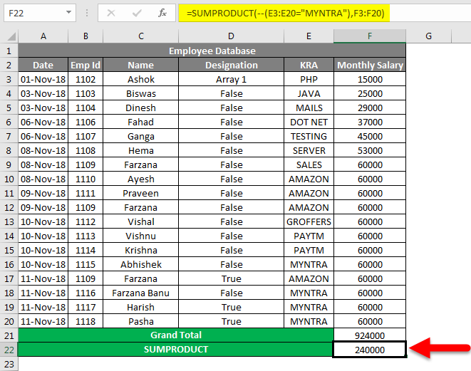
- In the above screenshot, we have used the SUMPROODUCT function with the first part of the array as (–) double negative because Excel will usually convert this as TRUE and FALSE values where TRUE=1 and False =0
- The second part of an array will look for G4:G21=”MYNTRA.”
- The third part of an array will look for the content values from H4:H21.
- Press the Enter key; we will get the output as 24000, shown as a result in the screenshot below.
Let’s see how the SUMPRODUCT function works with the (–) double negative values.
This SUM PRODUCT function will check the two arrays; if the given value is TRUE, it will take multiple with 1, and if the given value is false, it will multiply with 0 with the below calculation.
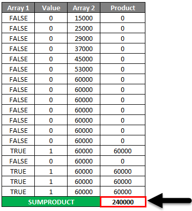
SUMPRODUCT function checks for the first array in the G column if the KRA is “MYNTRA,” Excel will consider this as TRUE with the value 1, i.e. =1*6000=6000. If the array in the G column is not “MYNTRA”, excel will consider this FALSE with 0, i.e. 0*6000=0.
Example #4 – Using SUMPRODUCT as COUNT Function
In this example, we will see how the SUMPRODUCT function works as a COUNT function.
Consider the same employee database where we need to count the number of AMAZON employees from the database given in example 3 by following the following steps.
- Create a new row for the count.
- Apply the SUMPRODUCT function =SUMPRODUCT (–(G4:G21=”AMAZON”)) as shown in the below screenshot.
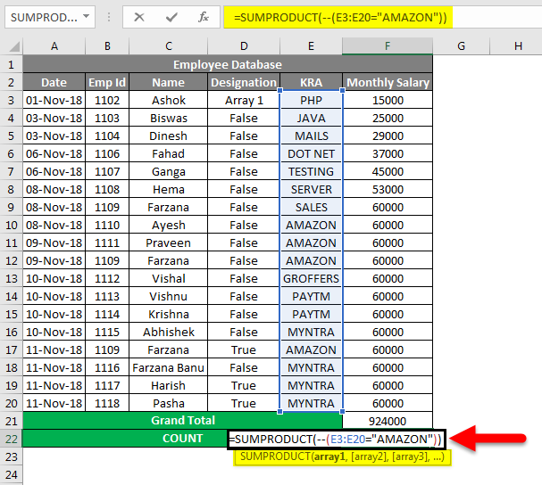
- In the SUMPRODUCT function, we can see that we have applied a (–) double negative to represent the value as TRUE or FALSE.
- The first part of an array will check in the G column if the KRA is AMAZON Excel will treat it as 1 (TRUE), or else Excel will treat it as 0 (FALSE)
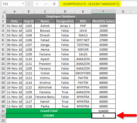
- Click the Enter key to get the number of counts for Amazon employees as four, which is shown as a result in the screenshot below.
Things to Remember
- SUM product will normally accept 255 arguments.
- SUMPRODUCT can use in functions like VLOOKUP, LEN, and COUNT.
- SUMPRODUCT function will throw and #VALUE! Error if the array dimension values are not in the same range
- The SUMPRODUCT function can also use as a COUNT function.
- In the SUMPRODUCT function, if we simply provide only one array value, the SUMPRODUCT function will just sum the values as output.
Recommended Articles
This has been a guide to SUMPRODUCT Function with Multiple Criteria in Excel. Here we discussed SUMPRODUCT Function with Multiple Criteria in Excel and how to use SUMPRODUCT Function, practical examples, and a downloadable Excel template. You can also go through our other suggested articles –
