Updated August 23, 2023
COUNTIF Formula in Excel
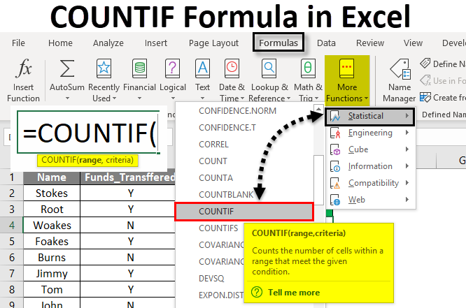
COUNTIF Formula in Excel is an inbuilt or pre-built integrated function that is categorized under the statistical group of formulae.
Excel COUNTIF Formula counts the number of cells within a specified array or range based on a specific criterion or applied condition.
Below is the Syntax of the COUNTIF Formula in Excel :
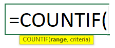
The COUNTIF Formula in Excel has two arguments, i.e., range and criteria.
- Range: (Required & Compulsory argument): The range or array of cells on which the criteria should be applied. Here array or range should be mentioned as, e.g., C1:C12.
- Criteria: (Required & Compulsory argument)) It is a specific condition that will be applied to the cell values presented by the range of cells. It indicates the Count IF formula “what cells need to be counted” here. There is a limitation of the criteria argument in the COUNTIF Formula, i.e., If the text string in the criteria argument contains greater than 255 characters in length or more than 255 characters. Then it returns #VALUE! Error.
Note: It can be either a cell reference, text string, or logical or mathematical expression.
- A named range can also be used in the COUNTIF formula.
- In the Criteria argument, Non-numeric values compulsorily should always be enclosed within double quotes.
- Criteria argument is case-insensitive, where it can consider any text case, whether proper or upper, or lower case.
- In the Excel COUNTIF formula, the below-mentioned arithmetic operators can also be used in the criteria argument
= Equal to
< Less Than
<= Less than or equal to
> Greater Than
>= Greater than or equal to
<> Less than or greater than
How to Use COUNTIF Formula in Excel?
COUNTIF Formula in Excel is very simple and easy to use. Let’s understand the working of the COUNTIF Formula in Excel with some examples.
Excel COUNTIF Formula – Example #1
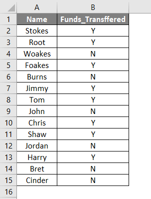
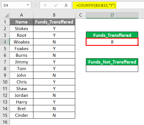
In the following example, the Table contains the company employee’s name in column A (A2 to A15) & funds transferred status in column B (B2 to B15). Here I need to find out the count of two parameters, i.e., funds transferred & funds not transferred in the dataset range (B2 to B15).
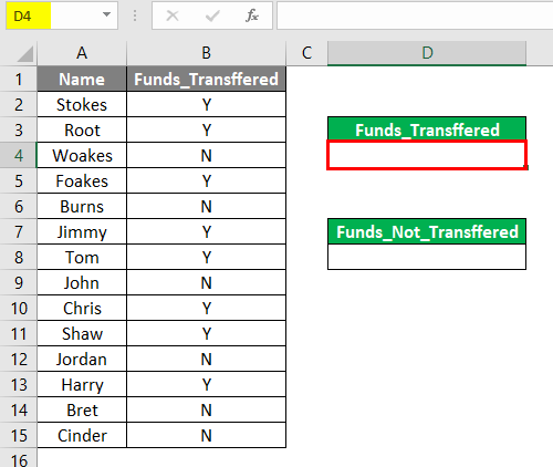
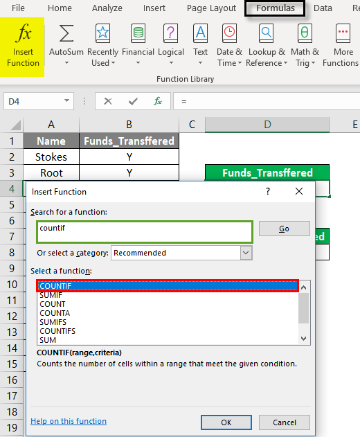
- Let’s apply the COUNTIF function in cell D4. Select cell D4 where the COUNTIF formula needs to be applied.
- Click or select an Insert Function (fx) button in the formula toolbar; a dialog box will appear, where you need to enter or type the keyword countif in the Search for a function box. The COUNTIF formula will appear in the Select a function box. Double click on the COUNTIF formula.
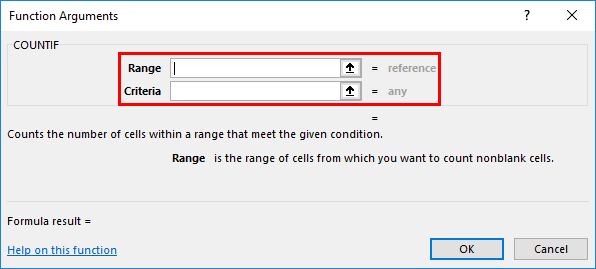
- A function argument dialog box appears where syntax or arguments for the COUNTIF formula needs to be entered or filled. i.e.,=COUNTIF (Range, Criteria)
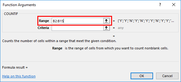
- Range: It is a range of cells where you want to count. The content or array is from B2 to B15, So select the column range. i.e., B2:B15
- Criteria: It is a condition or criteria where you insert the COUNTIF function, which cells need to be counted, i.e., “Y” (here, we need to find out the count of an employee who has received some funds). Click OK after entering both range & criteria arguments. =COUNTIF (B2:B15,”Y”)
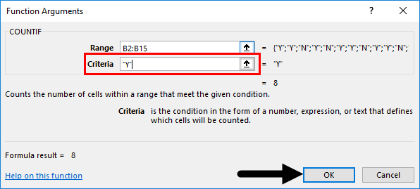
- The COUNTIF formula returns the count of an employee who has received funds, i.e., 8 from the dataset range (B2:B15). Here, the COUNTIF formula returns a count. 8 within a defined range. It means 8 employees have received funds.
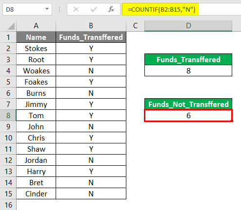
- Suppose I want to determine the number or count of employees who have not received funds. I just need to change the criteria argument, i.e., instead of “Y”, I need to use “N” =COUNTIF (B2:B15, “N”)
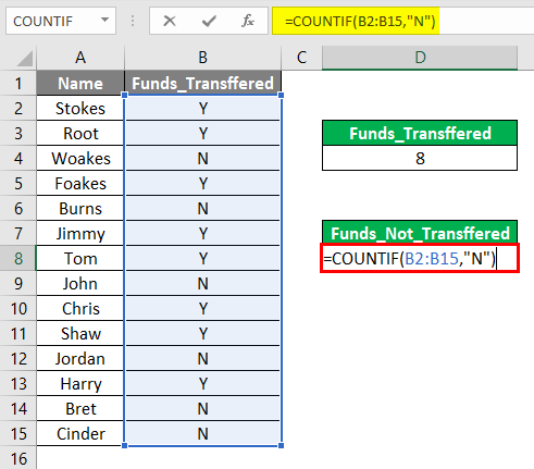
- The COUNTIF formula returns the count of an employee who has not received a fund, i.e., 6 from the dataset range (B2:B15). Here, the COUNTIF formula returns a count of 6 within a defined range. It means six employees who haven’t received funds.
Excel COUNTIF Formula – Example #2
With Arithmetic Operator in criteria argument
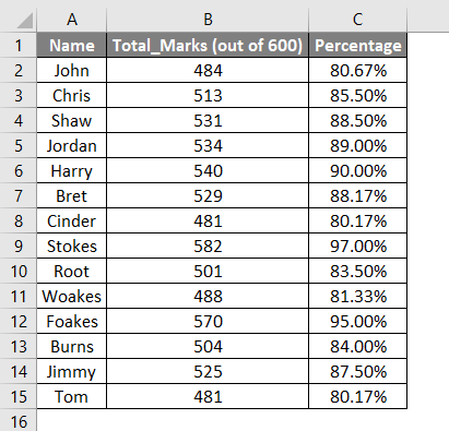
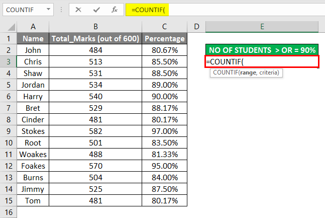
In the second example, the Table contains the student’s name in column A (A2 to A15), the Total marks scored in column B (B2 to B15), and their percentage in column C (C2 to C15); here, I need to find out the count or number of students who have scored more than or equal to 90% in a dataset range (C2 to C15).
- We can apply the COUNTIF formula with an arithmetic operator in cell E3. i.e.,=COUNTIF (Range, criteria)
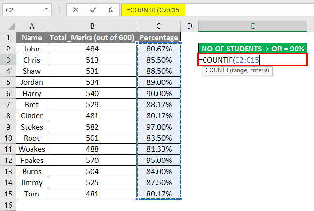
- Range: It is a range of cells where you want to count. The range or array is from C2 to C15, So select the column range. i.e. C2:C15.
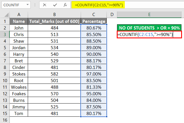
- Criteria: It is a condition or criteria where you inform the count of function, which cells need to be counted, i.e. ,”>=90%” (Here, I need to find out the count or number of Students who has scored more than or equal to 90% in a dataset range (C2 to C15)).
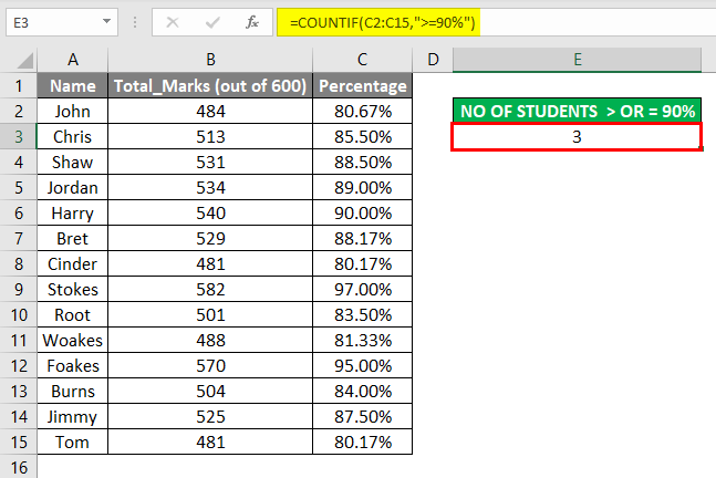
- Here, the =COUNTIF (C2:C15,” >=90%”) formula returns a value of 3, i.e., No of Students who have scored more than or equal to 90% in a dataset range (C2 to C15).
Things to Remember About COUNTIF Formula in Excel
The Wildcard characters can also be used in the Excel COUNTIF formula (in the criteria argument) to get the desired result; Wildcards help out in partial matching.
The three most commonly & widely used wildcard characters in the Excel COUNTIF formula are
- Asterisk (*): To match any trailing or leading characters sequence. E.g., Suppose you want to check all cells in a range containing a text string beginning with the letter “T” and ending with the letter “e”, You can enter the condition or criteria argument as “T*e”.
- tilde (~): To find an actual question mark or asterisk. E.g., Suppose you want to match all the cells in a range containing Asterisk (*) or Question mark (?) in the text, then tilde (~) is used in condition or criteria argument as “*~*shirt*” E.g., Red*shirt Green shirt.
In the above example, it will track the Red*shirt because it contains Asterisk (*) character in between
Asterisk (*) usage examples
TOR* Finds the text containing or Starting with TOR
*TOR Finds the text containing or Ending with TOR
*TOR* Finds the text Containing the word TOR
- Question mark (?): Used to identify or track any single character. e.g., Suppose you want to track “shirts” words or words ending with “S” in the below-mentioned example, then in the criteria argument, I need to use “shirt?”. It will result in the value 1.
Redshirts
Green shirt
Recommended Articles
This has been a guide to COUNTIF Formula in Excel. We discuss how to use COUNTIF Formula in Excel, practical examples, and a downloadable Excel template. You can also go through our other suggested articles –
