VLOOKUP with Sum in Excel (Table of Contents)
VLOOKUP with Sum in Excel
Vlookup with Sum function in Excel is used to Sum the numbers from the looked up range if the selected range matches the lookup value. We can choose multiple columns from the table where we want to Sum the values. For example, we have a table with sales data for fruits and different months’ sales in different columns. Then using Vlookup with the Sum function will return the sum of any selected lookup cell containing the fruit name, which will sum up the numbers from all the selected columns.
Vlookup in Excel Examples
Let’s look at some examples for lookup with a sum in Excel.
Vlookup with Sum in Excel – Example #1
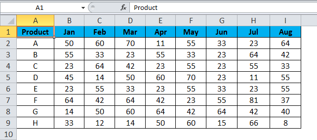
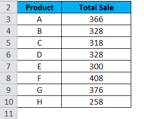
We have sales data for products named A, B, C,….H for 8 months. We need to see the total sale of any product in one shot. The data is shown below.
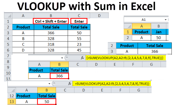
For that, we will be using Vlookup with Sum. First, we must identify the criteria we want to see as output. Consider seeing the output in a cell below in the same table. For that, go to the edit mode in any of the cells where the output will be printed. Now paste the formula =SUM(VLOOKUP(A2,’Sale Data’!$A$2:$I$9,{2,3,4,5,6,7,8,9},FALSE)) in edited cell.
And press Ctrl + Shift + Enter to see the output. The below screenshot shows the outcome of the applied formula.
Let’s do some experiments. As we can see in the below screenshot, it will not give the summed output of the entire selected row by just pressing the Enter key. This method will only reflect the first value of that row. For that, instead of Ctrl + Shift + Enter, press only Enter to exit from the cell.
This simple logic can summarize the formula which is given above.
=SUM(VLOOKUP(Lookup Value, Lookup Range, {2,3,4…}, FALSE))
- The lookup value is the fixed cell for which we want to see the sum.
- Lookup Range is the complete range or area of the data table from where we want to look up the value. (Always fix the Lookup range so that for other lookup values, the output will not get disturbed)
- {2,3,4… } are the column numbers for which we need to see the sum of the lookup cell.
- FALSE is the condition that says we need to see exact results; we can use TRUE as well, which is used to see the nearly approximate result. This can be used when our data is in discrete form.
This is the main feature, so Microsoft enabled the actual output to be seen only by pressing Ctrl + Shift + Enter keys. It shows that we only see the actual output when we correctly follow all the steps.
Vlookup with Sum in Excel – Example #2
Again, we will consider the same data shown in the screenshot below and see the products’ output in one shot.

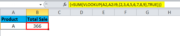
For this, identify a worksheet or place it in the same sheet where the output needs to be seen. I have chosen a separate sheet in the same file to see the output. And put the same logical formula as we have seen above as =SUM(VLOOKUP(A2,’ Sales Data’!$A$2:$I$9,{2,3,4,5,6,7,8,9}, FALSE)) and press Ctrl + Shift + Enter. We will get the output below screenshot.
As we can see, for all the products, their summed sales value for 8 months is here. You can cross-check as well if you want to compare the results.
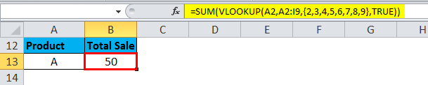
Let’s do one more experiment and compare; what will be the difference in output if we press Ctrl + Shift + Enter and only Enter key.
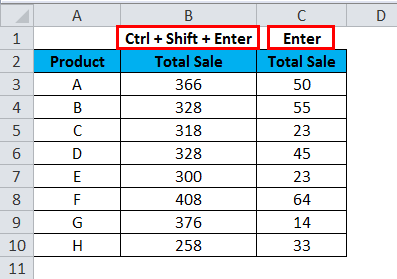
Here we have two output sets. By pressing the only Enter key, the formula prints only the first column data of the sales table, which is in column C. And by pressing Ctrl + Shift + Enter keys simultaneously, we get some of the subsequent product sales. And we can compare the data as well.
Pros of Vlookup with Sum
- Even if we modify the worksheet or Excel file after we apply the formula, the value will remain the same, and the results will not differ.
- Even if we have to press Ctrl + Shift + Enter to see the exact result, the outcome will get frozen, allowing us to have exact results.
Cons of Vlookup with Sum
- We need to select all the columns one by one by entering the column numbers in sequence, separated by commas after the lookup range, instead of selecting all the columns at the time, which we generally do in the simple Vlookup formula.
Things to Remember about the Vlookup with Sum in Excel
- Always freeze the lookup range by pressing the F4 key, which will put a $ sign on both sides. Which indicates that the cell or row, or range is fixed. And the value will not get changed, even if we change the range or sheet, or file location.
- Please keep track of columns that need to be considered in summing the count; sometimes, we may miss any number in the following.
- Once we exit from the cell, the Vlookup with the Sum formula itself gets enclosed in curve brackets {}, but if we wish to remove it, thus it will again get hidden in the same cell and reappear when we exit from it. This is the default function in Excel, which saves this formula.
- Always format the content before applying Vlookup with Sum; this will remove unwanted characters, spaces, and special characters to get the filtered sum value.
Recommended Articles
This has been a guide to VLOOKUP with Sum in Excel. VLOOKUP with Sum in Excel is a feature that automatically adjusts the width or height of a cell. Here we discuss how to use VLOOKUP with Sum in Excel, practical examples, and a downloadable Excel template. You can also go through our other suggested articles –
