Updated July 12, 2023
VLOOKUP with IFERROR (Table of Contents)
- How to Use IFERROR with VLOOKUP in Excel?
- Example #1: Replace #N/A Error with Customized Text
- Example #2: Replace #N/A Error with a Blank or Empty Cell
- Example #3: Return a Specific Value if Nothing is Found
- Example #4: Replace #N/A Error on a Fragmented Dataset
IFERROR with VLOOKUP in Excel
The IFERROR function combined with the VLOOKUP function in Excel allows you to return a specific customized text when the VLOOKUP encounters an error.
For example, you can replace the #N/A error with a customized text like “Data Not Found” or a blank cell. This powerful combination of IFERROR with VLOOKUP in Excel makes it easier to identify and handle the #N/A error when analyzing large amounts of data.
How to Use IFERROR with VLOOKUP in Excel?
Let’s say that you are looking for the city “Switzerland”, which is not present in the data, and you want to display “City Not Found.”
To use the VLOOKUP with the IFERROR function, follow these simple steps:
- In any cell, enter the Vlookup IFERROR formula =IFERROR(VLOOKUP(“Switzerland”, A2:B5, 2, FALSE), “City Not Found”).
- Press “Enter” to display the customized message, i.e., “City Not Found”.
You can also customize this formula for different data by replacing the following values:
- Replace Switzerland” with either the specific value you want to search for or the cell reference that contains that value.
- Replace “A2:B5” with the range that contains your data.
- Replace “2” with the column number you want to retrieve information from.
- You can use TRUE for an approximate match or FALSE for an exact match.
- You can replace “City Not Found” with any other personalized message.
Let’s understand the use of the IFERROR VLOOKUP in Excel with some examples.
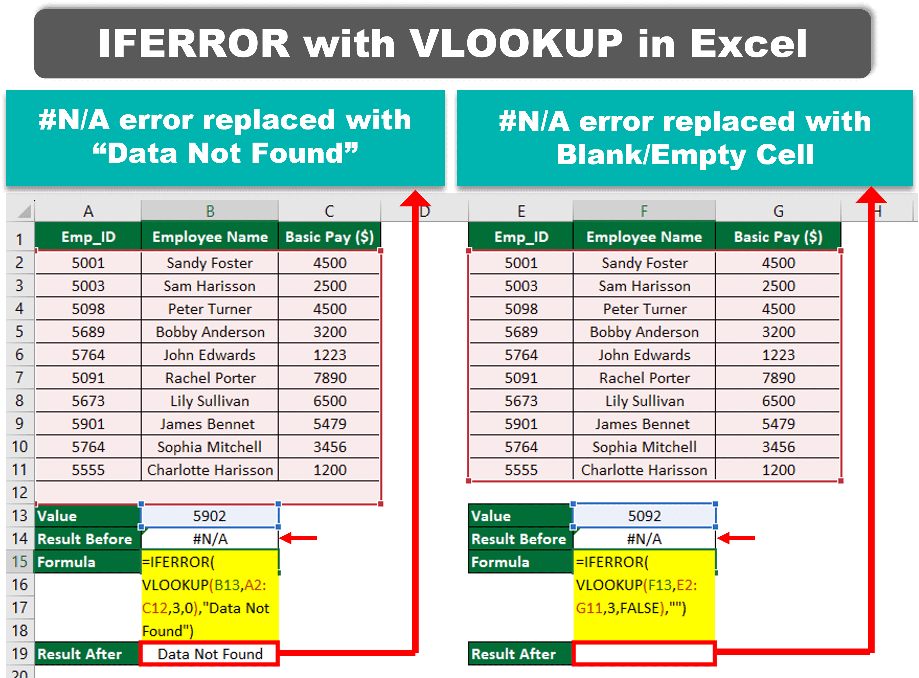
Example #1: Replace #N/A Error with Customized Text
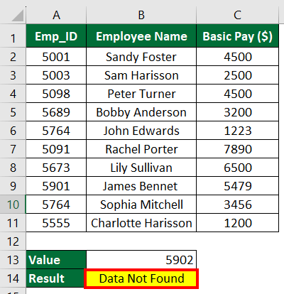
Consider the following data on the basic pay of employees in a company. Now, let’s assume you want to find out the salary of an Emp_ID 5902.
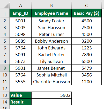
Solution:
First, let’s use the VLOOKUP function.
Step 1: Select Cell B14 and enter the formula:
Step 2: Press” Enter”.
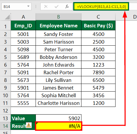
In the above table, we got a #N/A error.
It is because Emp_ID 5902 is not present in the table_array.
Therefore, to resolve this problem, we can combine the VLOOKUP function with the IFERROR function. We will replace the #N/A error with the customized text “Data Not Found”.
Step 3: To add customized text, select Cell B14 and enter the formula:
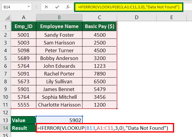
Step 4: Press “Enter”.
Result: The formula displays “Data Not Found” for Emp_ID 5902 instead of an error.
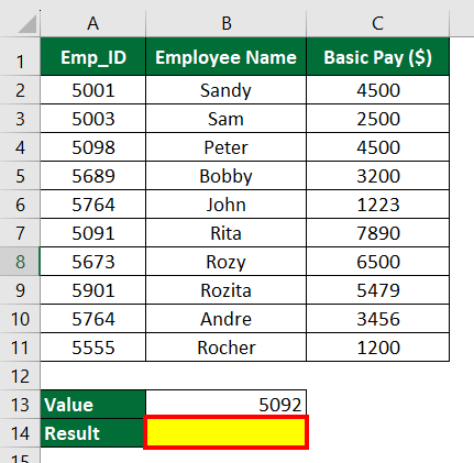
Example #2: Replace #N/A with a Blank or Empty Cell
In this example, we will see how to use IFERROR with VLOOKUP in Excel to return a blank instead of a #N/A error.
Solution:
Step 1: Select Cell B14 and enter the formula:
Note: Using the empty string (“”) in this formula will help achieve a blank cell.
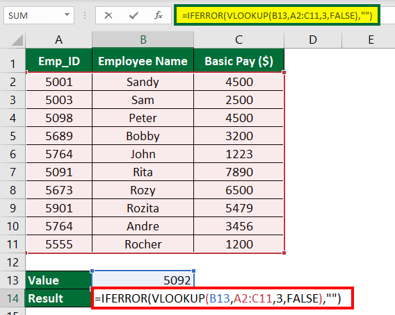
Step 2: Press “Enter”.
Result: Cell B14 is “Blank“.
Example #3: Display a Specific Value if Nothing is Found
Consider an e-commerce company that provides contact numbers on its website for different available services. However, if a user searches for a service that is not available, the default action is to display the customer care number.
So, let’s explore how we can display the customer care number when a user searches for “Order Assistance,” which is unavailable on the website.
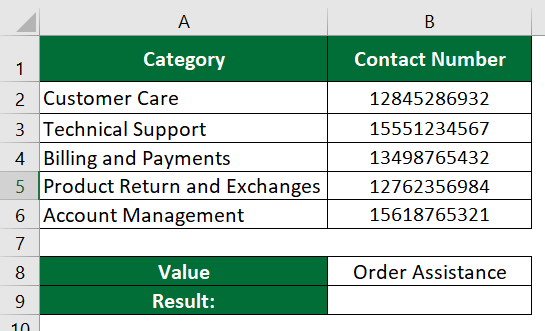
Solution:
Step 1: Select Cell B9 and enter the formula:
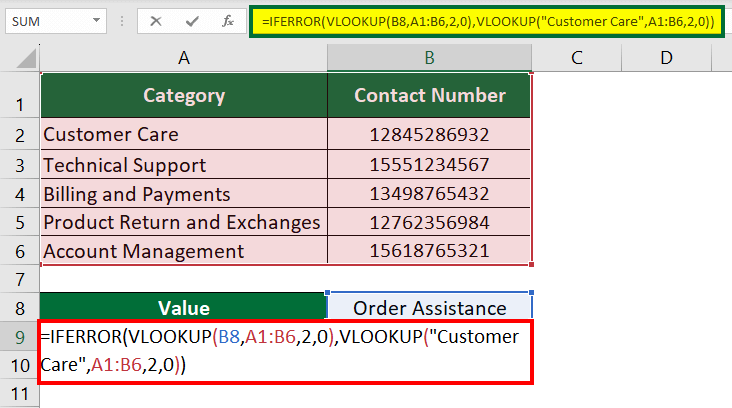
Step 2: Press “Enter” to display the output in Cell B9.
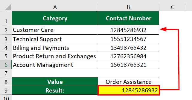
Result: The formula displays the contact number of “Customer Care” for order assistance.
Note:
=IFERROR(VLOOKUP(B8,A1:B6,2,0),VLOOKUP(“Customer Care”,A1:B6,2,0))
The first VLOOKUP function failed to find “Order Assistance” in this formula. Therefore, the formula automatically moved to the second VLOOKUP function and retrieved the customer care contact number.
Example #4: How to use IFERROR with VLOOKUP on a Fragmented Dataset?
This method will teach you to use IFERROR with VLOOKUP in Excel for fragmented datasets. Fragmented datasets mean that the data is present in multiple tables (instead of a single table).
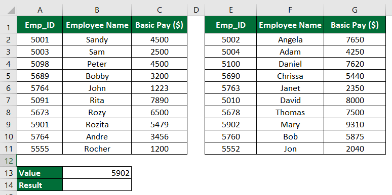
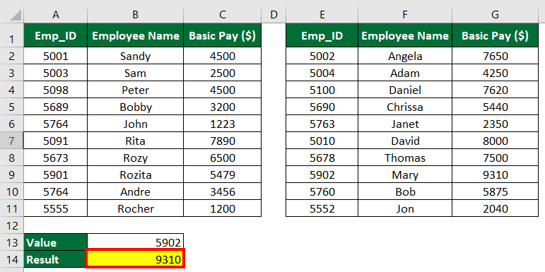
Consider the data below, where two tables are in the same worksheet. Here, you have to find out the basic pay for Emp_ID 5902.
Solution:
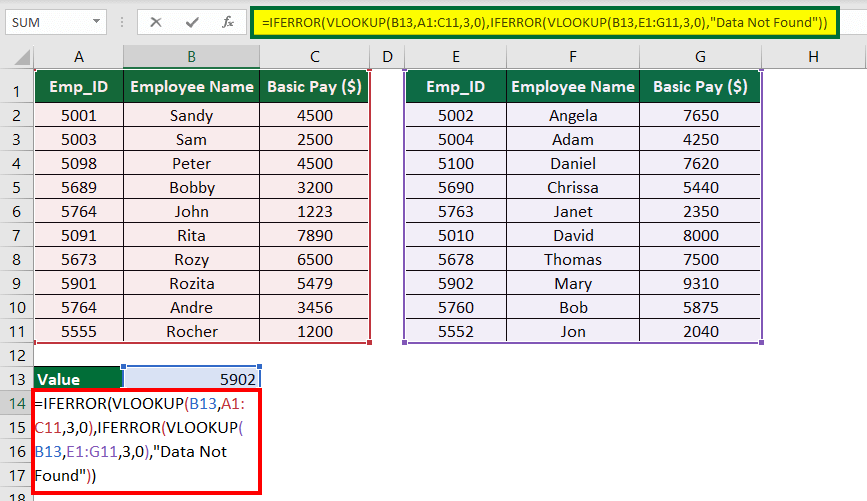
Step 1: Select Cell B14 and enter the formula:
Explanation of the formula:
=IFERROR(VLOOKUP(B13,A1:C11,3,0),IFERROR(VLOOKUP(B13,E1:G11,3,0),”Data not Found))
The formula states that the VLOOKUP function will check the lookup_value (B13) in the first table (A1:C11), and if the value is not found, then it will check in the second table (E1:G11). If the lookup_value is not found in both the tables, then the formula should display “Data not Found”.
Step 2: Press “Enter”.
Result: The formula display “9310″ in Cell B14.
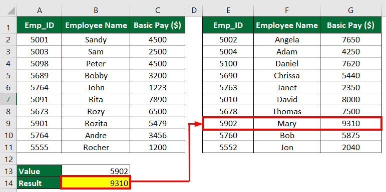
The formula fetched the result from the 2nd table, as shown below.
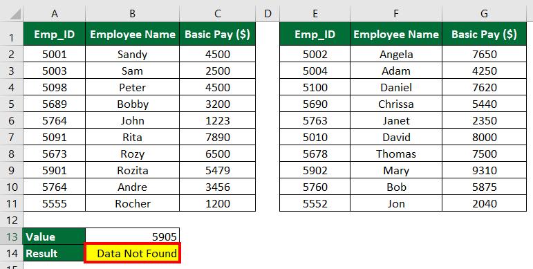
Suppose you search for Emp_ID 5115, which is not present in the data. Here, the formula will display “Data Not Found”, as shown below.
Recommended Articles
This article is a step-by-step guide on how to use IFERROR with VLOOKUP in Excel. Here we discuss in detail how to use IFERROR with VLOOKUP in Excel to replace #N/A error with customized text, blank cells, etc., along with practical examples. You can also review our other suggested articles:
