Updated May 3, 2023
Excel CHOOSE Function
Choose function in Excel returns a value from the selected list or array from any specific position. In simple language, we choose a function that returns a value based on the given position from the set available list of values. This function can be used in Excel worksheets or as VBA functions.
Formula:
Below is the CHOOSE Formula in Excel :
The CHOOSE formula has the following arguments:
- Index_num = The position of a value for which we are looking. It will always be a number between 1 and 254.
- Value 1 = The first value/list from which to choose.
- Value 2[optional] = The second value/list from which to choose.
In choose function, the Values parameter can be the cell references or the cell range. If Index_num is 1, then it will return Value 1.
Explanation of CHOOSE Function in Excel
When looking for a value corresponding to the index number or applying the Vlookup function, we realize that we have to pick the data from the left side as the Vlookup function works on the right side of the lookup value. Utilizing Excel’s CHOOSE function will allow you to tackle these issues. Here we will discuss some examples for solving the above problems.
How to Use CHOOSE Function in Excel?
Let’sLet’s take a few CHOOSE functions in Excel examples before using the Choose function workbook:
Example #1
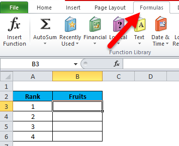
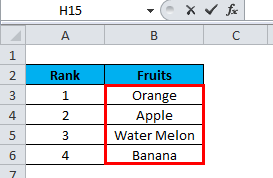
Exat’s suppose; We have ranks from 1 to 4 and fruits Orange, Apple, Water Melon, and Banana. Now in the result, we want to rank 1, it should be Orange, rank 2, it should be Apple, and so on.
For this problem, we will use the choose function.
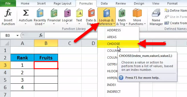
- Click on the Formulas tab.
- Then click on lookup and reference and select CHOOSE Function.
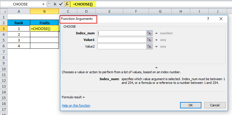
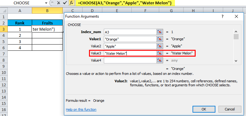
- In cell B3, we wrote =choose then bracket open and click on insert function. It will open a function arguments dialog box as per the below screenshot.
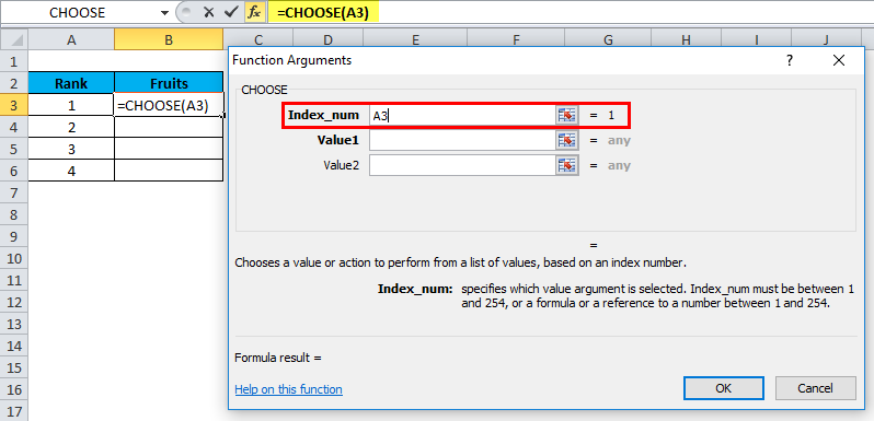
- In Index_num – select A3 cell for which we are looking value.
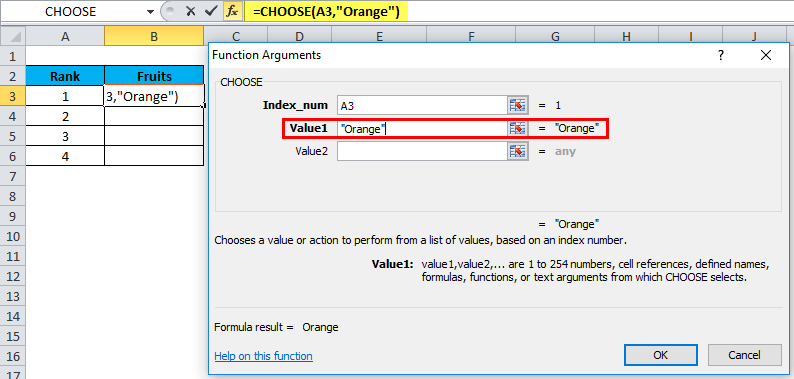
- In Value 1 – Pass First list value, i.e. Fruit name Orange. It automatically takes the parameter as text in double quotes.
- In Value 2 – Pass the Second fruit named Apple.
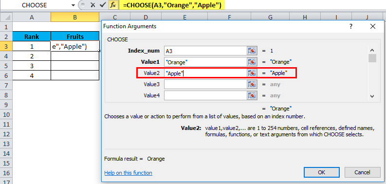
- In Value 3 – Pass the Third fruit name Water Melon.
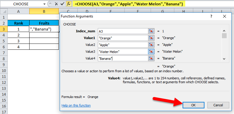
- In Value 4 – Pass the Fourth fruit name the Banana.
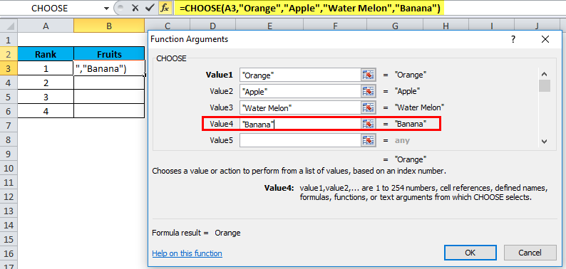
- Click on ok.
It will give the below result:
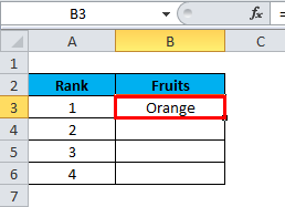
Drag & drop the value from B3 to B6, and it will produce the below results:
Example #2
Suppose you have the below list and you want to pick a value to exist on the 3rd position from the below list:
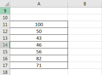
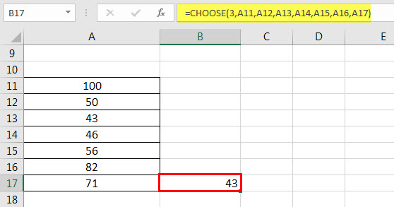
Now, you can use the formula =CHOOSE(3, A11, A12, A13, A14, A15, A16, A17)
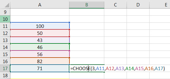
The result is 43.
Example #3
We also can pass the range in place of values. Please see the below example:
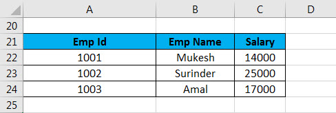
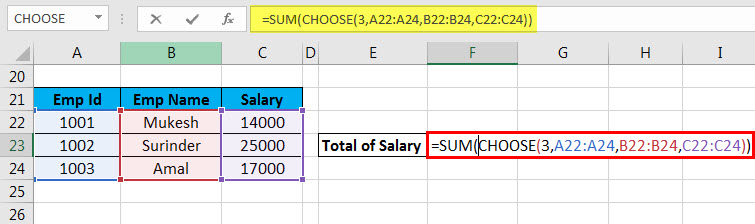
=CHOOSE(3, A22: A24, B22: B24, C22: C24) – we have taken the first argument as 3 because we want to see the total salary, which is the 3rd column in the above data. The above data is company employee data. Now we want to know the sum of the salary given by the company. Here we will use the choose function with the sum function.
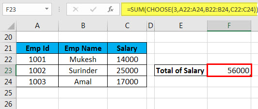
The result is 56000.
3rd index_num will choose the value from the 3rd range. If we pass 2nd as index_num, then it will choose the value from the 2nd range.
Example #4
We are taking an example of an XYZ company employee.
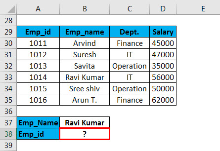
In the above example, we want to pick the Emp_id corresponding to the Emp_name. Here we will apply the Vlookup function along with CHOOSE function. Syntax is:
=VLOOKUP(G30, CHOOSE({1, 2,3, 4}, $B$30:$B$35, $C$30:$C$35, $D$30:$D$35, $A$30:$A$35), 4, FALSE)
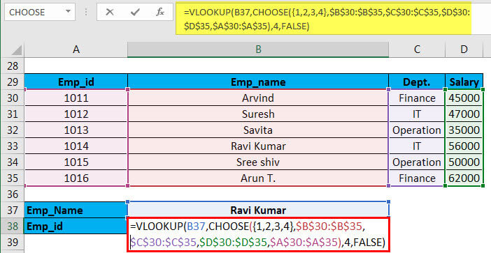
Here we pass an array at the place of the first argument in the CHOOSE function. Index 1 indicates Column B, Index 2 indicates Column C, Index 3 indicates Column D and Index 4 indicates Column A.
The result is 1014:
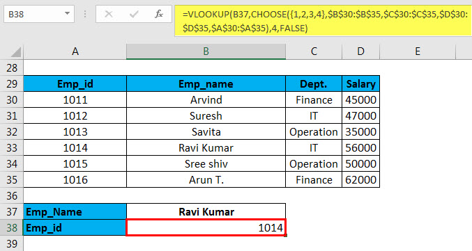
This method is also called the Left lookup formula with Lookup Function.
Recommended Articles
This has been a guide to CHOOSE function in Excel. Here we discuss the CHOOSE Formula in Excel and how to use CHOOSE function in Excel, along with practical examples and a downloadable Excel template. You can also go through our other suggested articles –
