Updated May 9, 2023
Excel SUMIFS with Dates (Table of Contents)
SUMIFS with Dates in Excel
SUMIFS is an Excel function used to find conditional sums with multiple conditions. This is a function that adds values that meet multiple criteria. People mostly use logical operators to compare different conditions. The different criteria use logical operators such as greater than, less than, greater than, or equal to, less than or equal to, and not equal to. While processing a sales report or banking transactions, there will be situations to deal with dates. Here we may calculate the sum of product sales within a particular date or the sum of the sales done after a particular date etc. The SUMIFS will be used with dates in this condition. SUMIFS can be a plural form of SUMIF where single criteria will be checked in SUMIF and multiple in SUMIFS.
Syntax of the SUMIFS Function
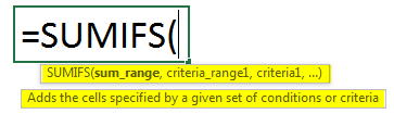
- Sum_range the cells to sum once the criteria are satisfied
- Criteria_range1 is the first range to be evaluated according to the criteria
- Criteria 1 is the first condition that should meet the criteria
- Criteria_range2, criteria 2 additional range and criteria for the specified range
The result will depend on all the criteria given. If anyone is not satisfied, it will not produce a result. SUMIFS works on AND logic, so if any criteria do not match, it won’t produce a result. The text and null values won’t be counted; only numeric values will be added to the sum.
How to Use SUMIFS with Dates in Excel?
When you have a single condition to check within a single range of cells, the SUMIF function is preferred. If the criteria are multiple and with a different range of cells, the SUMIFS function is used. Like the name, it will make the sum or range of cells only if the conditions are satisfied. With some examples, let’s understand how to use SUMIFS with Dates in Excel.
SUMIFS with Dates – Example #1
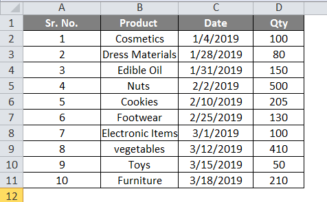
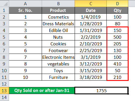
Below is the list of products shipped on different dates and Qty shipped. We need to find the sum of the shipped quantity for a particular period.
- The product list is given in column B, the Product shipped to date in column C, and Qty shipped in column D are below.
- Here we apply multiple conditions. We need to find the Qty shipped up to 18-Mar (consider as Today) and after Jan-31. Select column D13 and apply the formula to find the sum of Qty, which satisfies both conditions.
=SUMIFS (D2:D11, C2:C11,”<=”&TODAY (), C2:C11,”>=”&”01/31/2019″)
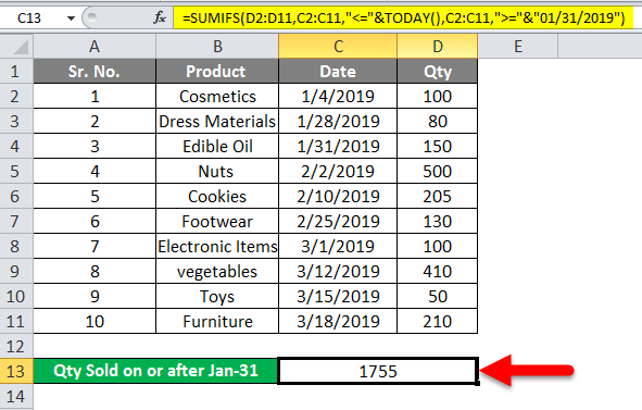
- Here D2: D1 is the range of Qty shipped C2: C1 is the range of dates shipped. Today () is the function to get the current day which is 18-3-2019. Logical operators are concatenated using the “&” symbol with the function or date.
- The first criteria will be “<=” & Today (). This will check the given dates with 18- Mar. Since this satisfies an entire column in the date, the Qty will be selected below to find the sum.
- For the second criteria, “>=” & “01/31/2019”, the date greater than or equal to 31-Jan the Qty shipped will select and make the sum as below.
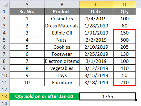
- The sum of Qty will come under both, from the shipped date of 1-31-2019 to 3-18-2019. And the sum is 1755, as shown in the 1st screenshot.
SUMIFS with Dates – Example #2
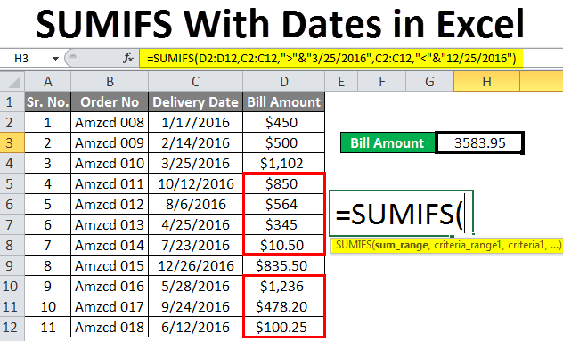
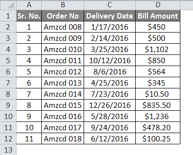
Another set of data is given below. Order number, date of delivery, and Bill Amount are given. We need to find the Bill amount after 3-25-2016 and before 12-25-2016
- Here we need to find the bill amount between the two mentioned dates. Select F3 and apply the formula
=SUMIFS (D2:D12, C2:C12,”>”&”3/25/2016”, C2:C12,”<“&”12/25/2016”)
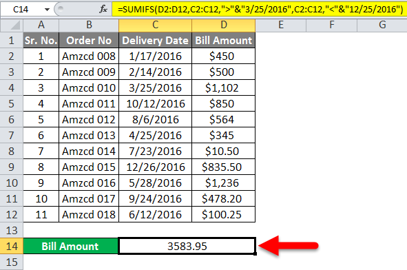
- D2: D12 is the sum_range and C2: C12 is the criteria range. The two measures are ‘>3/25/2016’ and ‘<12/25/2016’.
- Sum up the bill amount after ‘3/25/2016’ for the first criterion according to the requirements.
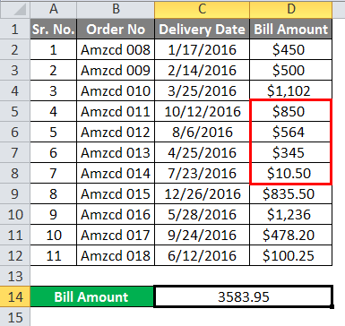
- And for the second criterion before ’12/25/2016′, the amounts will be selected as below.
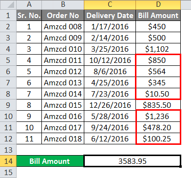
- So when both conditions are satisfied, the amount we will get is shown in the 1st screenshot. That is after 25-Mar and before 25-Dec. And the sum will be 3583.95.
SUMIFS with Dates – Example #3
In this example, we can use SUMIFS with blank and non-blank criteria.
- Order date and the delivery date of some products are given with Qty.
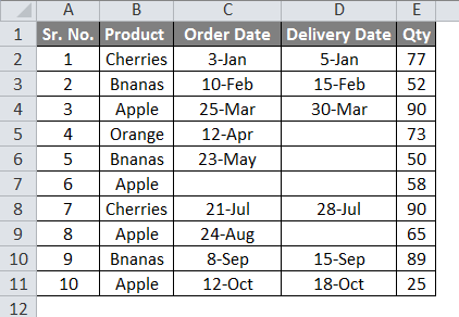
- We need to find the Qty of the Product not delivered yet and apply the formula in cell D13.
=SUMIFS (E2:E11, C2:C11,”<>”, D2:D11,”=”)
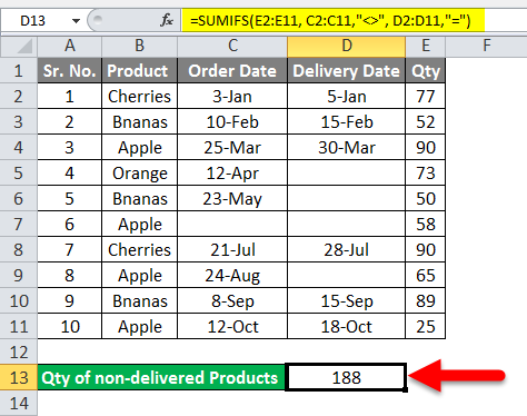
- In the first condition, ‘C2: C11,” <>”‘ we will select the non-empty cells in date order. And in the second condition, we will select the blank cells in the delivery.
- So both criteria satisfying cells will be as below.
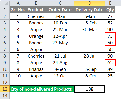
- So the sum of both criteria satisfying cells will be 188 in D13.
Things to Remember About SUMIFS with Dates
- The SUMIFs formula returns an error value’ #VALUE!’ when the criteria do not match the criteria range.
- Use the ‘&’ symbol to concatenate an Excel function with a criteria string.
- SUMIFS function works according to the AND logic, which means the range will be summed only if it meets all the given conditions.
- Whenever you enter an array formula that means a long formula, press Ctrl + Shift + Enter, enclosing your formula within a curly brace to help you easily manage the long formula.
- The answer will be ‘0’ when the criteria do not match.
Recommended Articles
This is a guide to SUMIFS with Dates in Excel. Here we discuss how to use SUMIFS Function with Dates in Excel, practical examples, and a downloadable Excel template. You can also go through our other suggested articles–
