Updated May 30, 2023
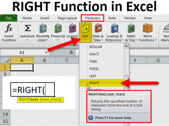
RIGHT Function in Excel
Right function in Excel, which is used to extract the cell values starting from the extreme right. We can also select the number of characters we must extract from the selected cell. This is quite helpful in extracting some portion of the text. For example, if a cell contains FIRST and we want to use the Right function here considering 3 characters to be extracted, we will get RST starting from the right as output.
RIGHT Formula in Excel:
Below is the RIGHT Formula in Excel.
Explanation of RIGHT Function in Excel:
A RIGHT Formula in Excel has two parameters: i.e., text and num_chars.
- Text: From the text that you want to extract specified characters.
- The number of characters you want to extract from the given text. [num_chars]: This is an optional parameter. If you do not provide any numbers by default, it will give you only one character.
Usually, a RIGHT function in Excel is used alongside other text functions like SEARCH, REPLACE, LEN, FIND, LEFT, etc…
How to Use RIGHT Function in Excel?
RIGHT Function in Excel is very simple and easy to use. A RIGHT function can be used as a worksheet function and a VBA function. Let us understand the working of the RIGHT function in Excel by some RIGHT Formula examples.
Example #1
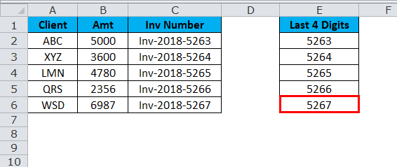
Look at the below data that contains invoice numbers. You need to extract the last 4 digits of all the invoice numbers using the RIGHT function in Excel.
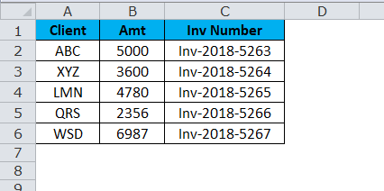
We can extract the last 4 digits of the above text using the RIGHT function in Excel.
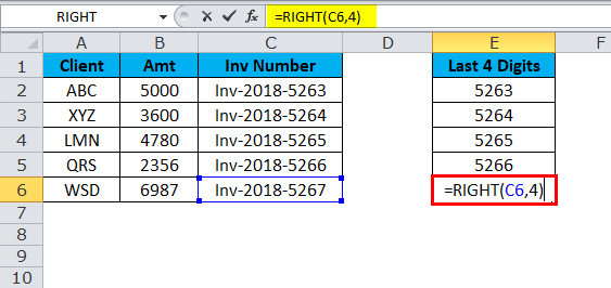
So the result will be :
Example #2
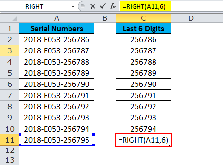
Assume you have serial numbers from A1 to A10 and must extract 6 characters from the right.
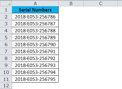
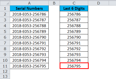
A RIGHT function will return the last 6 digits from the right end of the text.
Result is :
Example #3
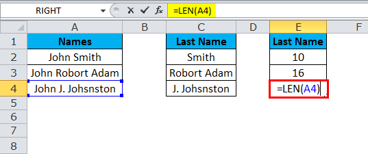
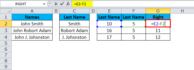
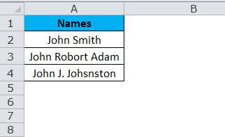
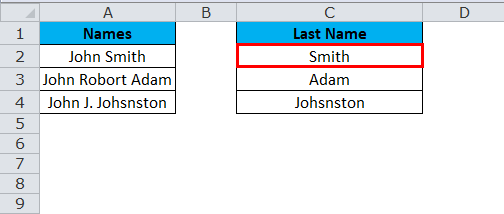
Below are the names of the employees, and you need to extract the Last Name separately.
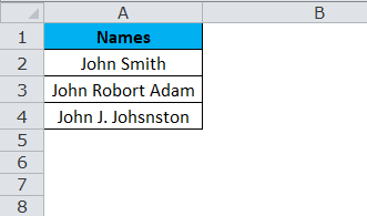
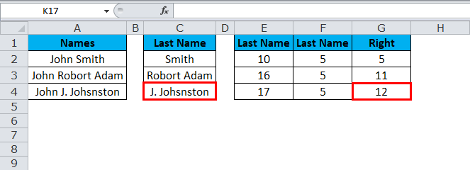
In the above example, we cannot just apply RIGHT with specified numbers because the last name of every employee is different. Here we need to use LEN & FIND function to determine the number of characters from the given text. For the first employee, the last 4 characters are 5, but for the second one, it is 11 (including space, i.e., Robert Adam), and for the third one, it is 12 (including space, i.e., J. Johnston).
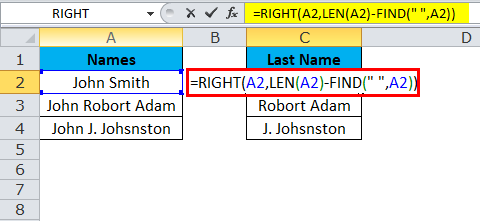
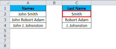
So the result will be :
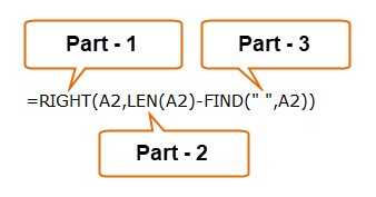
Part 1: This part determines the desired text that you want to extract from the characters.
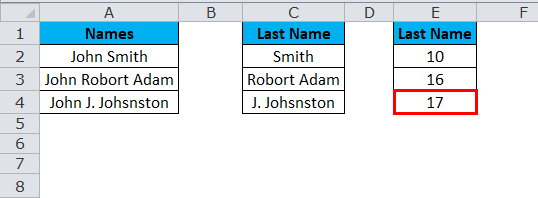
Part 2: LEN function will give you the total number of characters in the list. We will see the detailed article on LEN in the upcoming articles.
Result is :
Part 3: The FIND function determines from which number space begins, i.e., The End of the first name. We will see the detailed article on FIND in the upcoming articles.
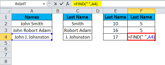
Result is :
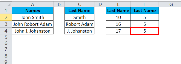
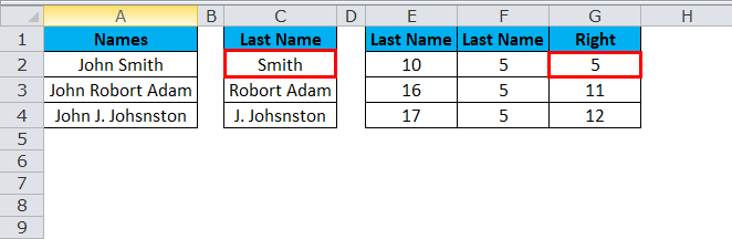
Len gives 10 characters and Finds 5 for the first employee. That means LEN – FIND (10 – 5) = 5 characters from the right side.
The result will be Smith.
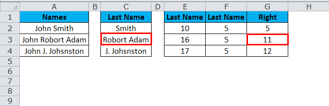
Len gives 16 characters, and Find gives 5 characters for the first employee. That means LEN – FIND (16 – 5) = 11 characters from the right side.
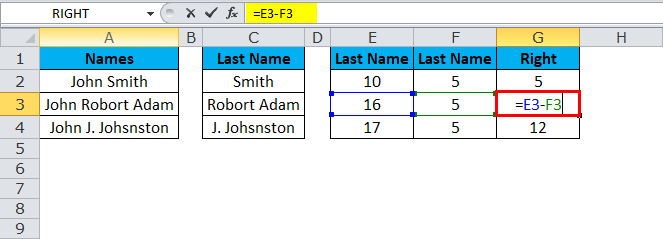
The result will be Robert Adam.
Len gives 17 characters, and Find gives 5 characters for the first employee. That means LEN – FIND (17 – 5) = 12 characters from the right side.
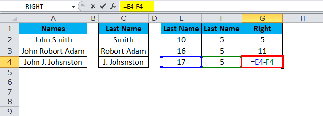
The result will be J. Johnston.
Example #4
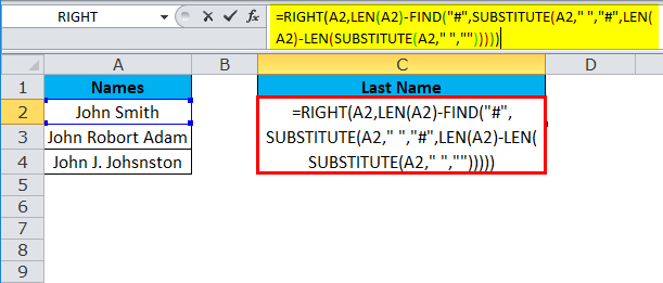
Let us consider the same example from the above. Name the employees, and you need to extract the Last Name separately. i.e., only ADAM, not ROBORT ADAM.
This is done using LEN, FIND, and SUBSTITUTE formulas alongside the RIGHT function in Excel.
The first SUBSTITUTE function will replace the space (““) with “#,” and then LEN, a function, will deduct the space character number from the SUBSTITUTE function to get only the last name characters.
So the result will be :
Example #5
From the below table, extract the last number until you find a space.
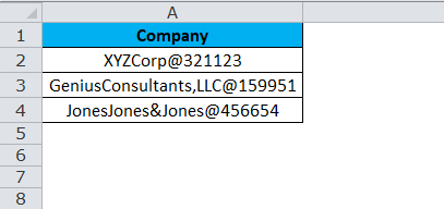
This is a bit of complex data, but we can still extract the last characters using the RIGHT Function in Excel and the FIND function.
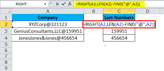
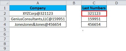
So the result will be :
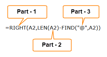
Part 1: This part determines the desired text that you want to extract from the characters.
Part 2: LEN function will give you the total number of characters in the list.
Part 3: The FIND function determines from which number “@” begins.
Example #6
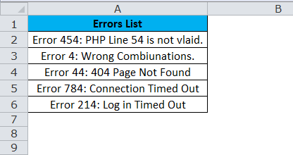
Below are the errors find out while you are working on the web-based software. You need to extract the substring after the last occurrence of the delimiter.
This can be done by combining LEN, SEARCH & SUBSTITUTE, and the RIGHT function in Excel.
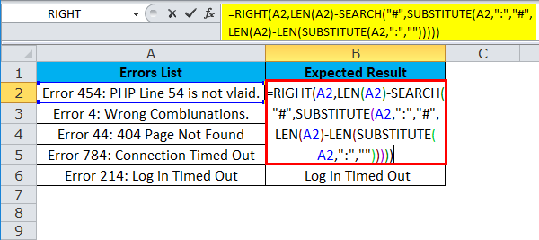
- The first step is to calculate the total length of the string using the LEN function: LEN(A2)
- The second step is to calculate the length of the string without delimiters by using the SUBSTITUTE function that replaces all occurrences of a colon with nothing: LEN(SUBSTITUTE(A2, “:”,”))
- Lastly, we subtract the length of the original string without delimiters from the total string length: LEN(A2)-LEN(SUBSTITUTE(A2, “:”,”))
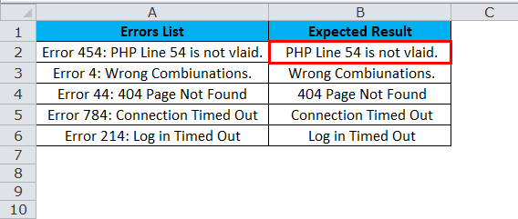
So the result would be:
Example #7
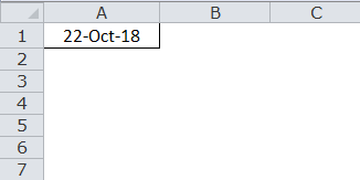
RIGHT Function in Excel does not work with Dates. Since the RIGHT function is a text function, it can extract numbers too, but it does not work with dates. Assume you have a date in cell A1 “22-Oct-18.”
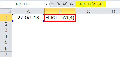
Then we’ll try to extract the year with the formula.
The result would be 3395.
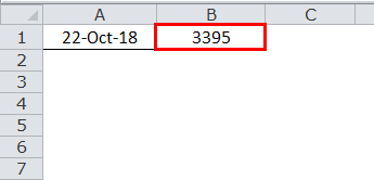
In Excel, ideology 3395 means 2018 if the format is in Dates. So RIGHT function in Excel will not recognize it as a date but, as usual, as a number only.
VBA RIGHT Function
In VBA, also we can use the RIGHT function. Below is a simple illustration of the VBA right function.
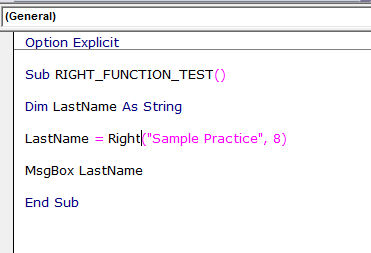
If you run the above code, it will give you the below result.
Things to Remember
- Number formatting is not part of a string and will not be extracted or counted.
- Right Function in Excel is designed to extract the characters from the right side of a specified text.
- If the user does not specify the last parameter, it will take 1 by default.
- Num_chars must be greater than or equal to zero. If it is a negative number, it will throw the error as #VALUE.
- A RIGHT function will not give accurate results regarding date formatting.
- In the case of complex data sets, you need to use other text functions like LEN, SEARCH, FIND, and SUBSTITUTE to get the Num_chars parameter.
Recommended Articles
This has been a guide to the RIGHT Function in Excel. Here we discuss the RIGHT Formula in Excel and How to use the RIGHT Function in Excel, along with practical examples and a downloadable Excel template. You can also go through our other suggested articles –
