What is Machine Learning Algorithms?
Computers can learn from data and make predictions without explicit programming through machine learning algorithms. They utilize statistical patterns and mathematical models to identify relationships and patterns within datasets, allowing for tasks like classification, regression, clustering, and more. These algorithms play a crucial role in various fields, including artificial intelligence, data science, and predictive analytics, enabling automated decision-making and pattern recognition in diverse applications such as image recognition, natural language processing, and recommendation systems.
Table of Contents
Importance of Machine Learning Algorithms
Machine Learning Algorithms are essential because they power the decision-making capabilities of artificial intelligence systems. These algorithms enable machines to learn from data, recognize patterns, make predictions, and automate tasks without explicit programming. Their significance lies in their capacity to extract valuable insights from vast datasets, optimize processes, enhance application personalization, and even contribute to scientific advancements. In fields like healthcare, finance, and autonomous driving, they drive innovation by facilitating predictive modeling and improving efficiency. In essence, Machine Learning Algorithms underpin the transformative potential of AI, making them indispensable for tackling complex problems and shaping the future of technology and industry.
Types of Machine Learning Algorithms
There are various ways to categorize types of machine learning algorithms, but they are typically grouped into classes based on their purpose. The primary categories include the following:
1. Supervised Learning
Supervised Learning is where you can consider an instructor who guides the learning. We have a dataset that goes about as an educator, and its job is to prepare the model or the machine. When the model is ready, it can begin settling on an expectation or choice when new information is given.
Example of Supervised Learning:
- You get a lot of photographs with data about what is on them, and after that, you train a model to perceive new photographs.
- You have a lot of data about house prices based on their size and location, and you feed it into the model and train it; then, you can predict the cost of other houses based on the data you feed.
- If you want to predict whether your message is spam or not based on your older message, you can predict whether a new message is spam.
2. Unsupervised Learning
The model learns through perception and discovers structures in the information. When the model receives a dataset, it subsequently finds examples and connections in the dataset by creating clusters within it. It can’t add marks to the bunch, similar to it can’t state this a gathering of apples or mangoes; however, it will isolate every one of the apples from mangoes.
Assume we displayed pictures of apples, bananas, and mangoes to the model, so it makes bunches and partitions the dataset into those groups in light of specific examples and connections. When you feed additional information to the model, it incorporates it into one of the existing clusters.
Example of Unsupervised Learning
- You have a lot of photographs of 6 individuals without data about who is on which one, and you need to isolate this dataset into six heaps, each with the photographs of one person.
- You have particles; some are medications, and parts are not; however, you don’t realize which will be which, and you need the calculation to find the medicines.
3. Semi-Supervised Learning
Semi-supervised learning involves calculating based on a mixture of named and unlabeled data. Normally, this blend will contain a limited quantity of named information and many unlabeled information. The fundamental method included is that the software engineer will first group comparable information utilizing an unaided learning calculation and afterward utilize the current named information to name the remainder of the unlabeled information. The ordinary use instances of such calculation have a typical property among them. Obtaining unlabeled information is generally modest, while naming the said information is over the top expensive. Naturally, one may envision the three kinds of learning calculations as Supervised realizing, where an understudy is under the supervision of an instructor at both home and school; unsupervised realizing, where an understudy needs to make sense of an idea himself; and Semi-Supervised realizing, where an educator shows a couple of ideas in class and gives inquiries as schoolwork which depend on comparable ideas.
Example of Semi-Supervised Learning
It’s outstanding that more information equals better quality models in profound learning (up to a specific point of confinement clearly, yet we don’t have that much information more often than not.) Be that as it may, getting marked information is costly. For example, if you need to prepare a model to distinguish winged animals, you can set up many cameras to take pictures of fowl. That is generally modest. Contracting individuals to mark those photos is costly. Consider the possibility that you have many images of winged animals; however, contract individuals to mark a small subset of the photos. As it turned out, rather than simply training the models on the marked subset, you can pre-train the model on the whole training set before tweaking it with the named subset, and you show signs of improvement execution along these lines. That is semi-supervised learning. It sets aside your cash.
4. Reinforcement Learning
A specialist can collaborate with the earth and discover the best result. It pursues the idea of hit and preliminary technique. The operator earns or incurs a point for a correct or incorrect answer and trains itself based on the positive reward points gained. Also, again, once prepared, it prepares to foresee the new information introduced to it.
Example of Reinforcement Learning
- Displaying ads, according to user likes and dislikes, optimizes for the long period.
- Know the ad budget used in real-time.
- Inverse reinforcement learning to know customers’ likes and dislikes better.
Popular Machine Learning Algorithms
There are currently numerous Machine Learning algorithms in the market, and it will only increase considering the amount of research done in this field. Linear and Logistic Regression are generally the first algorithms you learn as a Data Scientist, followed by more advanced algorithms.
Below is the list of the algorithms for Machine Learning, along with sample code snippets in Python:
1. Linear Regression
Linear regression is valuable for discovering the connection between two persistent factors. One is a predictor or autonomous variable; the other is a reaction or ward variable. It searches for measurable relationships, however, not a deterministic relationship. The connection between two factors is deterministic if one variable accurately expresses the other. For instance, utilizing temperature in degrees Celsius, it is conceivable to foresee Fahrenheit precisely. A factual relationship isn’t precise in deciding a connection between two factors. For instance, connection somewhere in the range of tallness and weight. The central thought is to get a line that best fits the information. The best-fit line minimizes the overall forecast error (all data points) as much as possible. The mistake is the separation between the point to the regression line.
As the name suggests, this algorithm could be used in cases where the continuous target variable is linearly dependent on the dependent variables.
It is represented by:
Where y is the target variable we are trying to predict, a is the intercept, and b is the slope, x is our dependent variable used to make the prediction. This is a Simple Linear Regression, as only one independent variable exists.
In the case of Multiple Linear Regression, the equation would have been:
Here, e is the error term, and a1, a2.. a (n) are the coefficients of the independent variables.
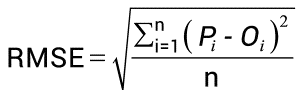
We use a metric to evaluate the model’s performance, which can be Root Mean Square Error (RMSE), calculated as the square root of the mean of the sum of differences between the actual and predicted values.
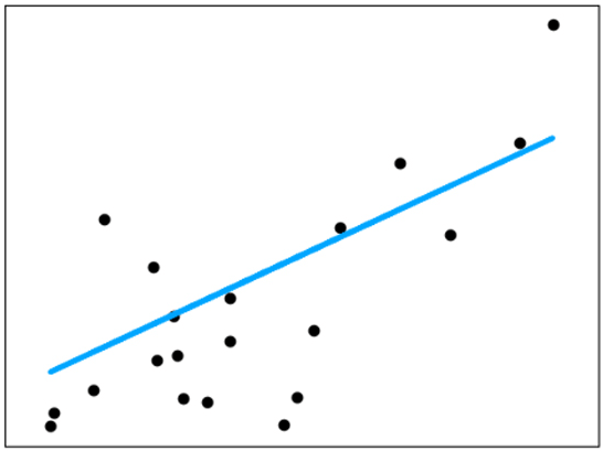
Linear Regression aims to find the best-fit line that would minimize the difference between the actual and the predicted data points.
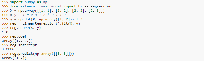
Linear Regression could be written in Python as below:
![]()
2. Decision Trees
A Decision tree is a decision-help gadget that uses a tree-like diagram or model of decisions and their potential outcomes, including chance-event results, resource costs, and utility. Explore the image to get a sentiment of what it resembles.
Used for classification and regression problems, the Decision Tree algorithm is one of the most simple and easily interpretable Machine Learning algorithms. Moreover, it is not affected by outliers or missing values in the data and could capture the non-linear relationships between the dependent and the independent variables.
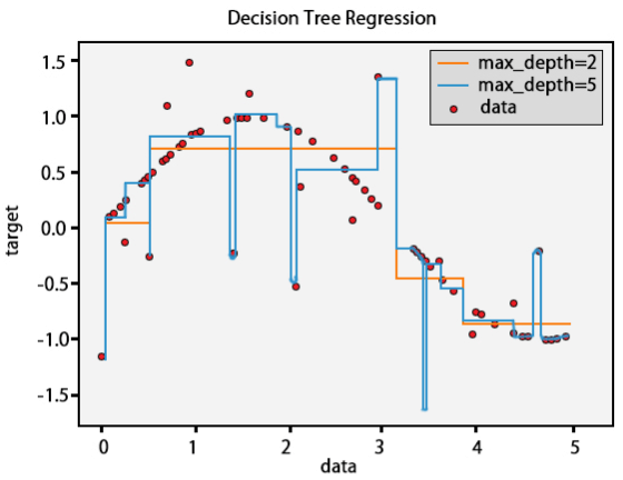
All features are considered to build a Decision Tree at first, but the feature with the maximum information gain is taken as the final root node based on which the successive splitting is done. This splitting continues on the child node based on the maximum information criteria, and it stops until all the instances have been classified or the data cannot be split further. Decision Trees are often prone to overfitting, and thus, it is necessary to tune the hyperparameters like maximum depth, minimum leaf nodes, minimum samples, maximum features, and so on. There is a greedy approach that sets constraints at each step and chooses the best possible criteria for that split to reduce overfitting. There is another better approach called Pruning, where the tree is first built up to a specific pre-defined depth, and then starting from the bottom, the nodes are removed if it doesn’t improve the model.
In sklearn, Decision Trees are coded as:
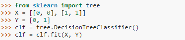
![]()
![]()
3. Naive Bayes Classification
Naive Bayes classification is a group of basic probabilistic classifiers dependent on applying Bayes’ theory with strong (unsophisticated) self-governance of the features of Naive Bayes. Some of the certifiable models are:
- To stamp an email as spam or not spam.
- Order a news story about innovation, governmental issues, or sports.
- Check a touch of substance imparting positive emotions or negative sentiments.
- Utilized for face acknowledgment programming.
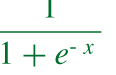
It works on the Bayes Theorem principle, which finds an event’s probability considering some true conditions.
Bayes Theorem is represented as:
The algorithm is called Naive because it believes all variables are independent and the presence of one variable doesn’t have any relation to the other variables, which is never the case in real life. As a result, naive Bayes could be used in Email Spam classification and text classification.
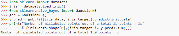
Naïve Bayes code in Python:
4. Logistic Regression
Logistic regression is a ground-breaking factual method for demonstrating a binomial result with at least one informative factor. It quantifies the connection between the absolute ward variable and at least one free factor by evaluating probabilities utilizing a logistic capacity, the combined logistic appropriation.
In terms of maintaining a linear relationship, it is the same as Linear Regression. However, unlike in Linear Regression, the target variable in Logistic Regression is categorical, i.e., binary, multinomial, or ordinal. Moreover, the choice of the activation function is essential in Logistic Regression as for binary classification problems, the log of odds in favor, i.e., the sigmoid function, is used.
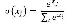
In the case of a multi-class problem, the softmax function is preferred as a sigmoid function takes a lot of computation time.
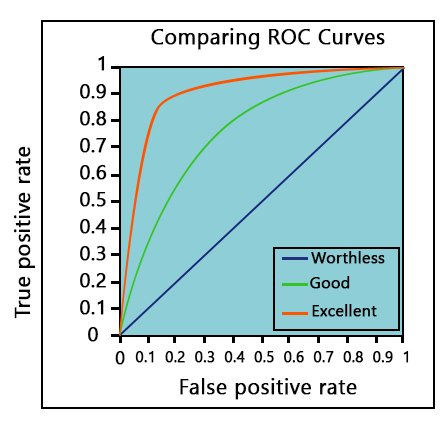
The metric used to evaluate a classification problem is Accuracy or the ROC curve—the more the area under the ROC, the better the model. For example, a random graph would have an AUC of 0.5. A value of 1 indicates the most accuracy, whereas 0 indicates the least accuracy.
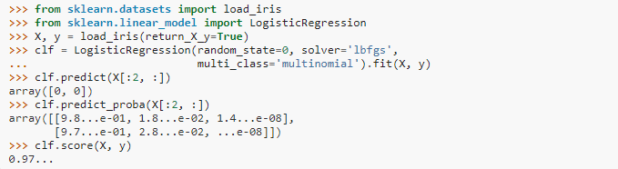
Logistic Regression could be written in learning as:

5. Ordinary Least Squares Regression
The least squares is a strategy for performing direct regression. Direct regression is fitting a line through a lot of focus. There are various potential procedures to do this, and the “ordinary least squares” system goes like this. You can draw a line, and after that, for all of the data centers, measure the vertical detachment between the point and the line and incorporate these up; the fitted line would be the place where this aggregate of partitions is as meager as could be normal in light of the current situation.
6. Clustering
Clustering is a significant idea with regard to unaided learning. It finds a structure or example in a gathering of uncategorized information for the most part. Clustering calculations will process your information and discover characteristic clusters(groups) if they exist in the information. You can likewise alter what number of bunches your calculations ought to distinguish. It enables you to alter the granularity of these gatherings.
There are various kinds of clustering machine learning algorithms you can use
- Selective (apportioning)
- Model: K-means
- Agglomerative
- Model: Hierarchical clustering
- Covering
- Model: Fuzzy C-Means
- Probabilistic
Clustering algorithm Types
- Hierarchical clustering
- K-means clustering
- K-NN (k nearest neighbors)
- Principal Component Analysis
- Solitary Value Decomposition
- Independent Component Analysis
1. Hierarchical Clustering
Hierarchical clustering is a calculation that constructs a pecking order of groups. It starts with every one of the information which is doled out to their very own bunch. Here, two close groups will be in a similar bunch. This calculation closes when there is just one group left.
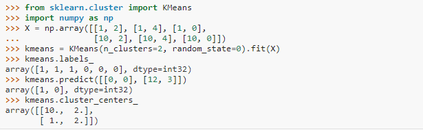
2. K-means Clustering
K means it is an iterative clustering calculation that encourages you to locate the most noteworthy incentive for each emphasis. At first, the ideal number of groups is chosen. In this clustering technique, you must bunch the information focusing on k gatherings. A bigger k means smaller gatherings with greater granularity, similarly. A lower k means bigger gatherings with less granularity.
The yield of the calculation is a gathering of “names.” It allows information to point to one of the k gatherings. In k-means clustering, each gathering is characterized by making a centroid for each gathering. The centroids are like the core of the bunch, which catches the focus nearest to them and adds them to the group.
K-mean clustering further characterizes two subgroups.
- Agglomerative clustering: This sort of K-means clustering begins with a fixed number of bunches. Then, it designates all information into an accurate number of groups. This clustering strategy doesn’t require the number of groups K as info. The agglomeration procedure begins by shaping every datum as a solitary bunch. Combining processes, this strategy utilizes some separation measures and lessens the number of bunches (one in every emphasis). In conclusion, we have one major group that contains every one of the articles.
- Dendrogram: Each level will speak to a conceivable bunch in the Dendrogram clustering technique. The tallness of the dendrogram demonstrates the degree of similitude between two joint bunches. The closer to the procedure’s base, the more comparable the finding of the gathering from the dendrogram, which isn’t characteristic and, for the most part, abstract.
So far, we have worked with supervised learning problems with a corresponding output for every input. Now, we would learn about unsupervised learning, where the data is unlabelled and needs to be clustered into specific groups. There are several clustering techniques available. However, the most common of them is the K-means clustering. In k-means, you need to set the number of clusters prior to maximizing variance in the dataset. Once the k is set, the centroids are initialized. The centroids are then adjusted repeatedly so that the distance between the data points within a centroid is maximum and the distance between two separate is maximum. Euclidean distance, Manhattan distance, etc., are some distance formulas used for this purpose.
The value of k could be found from the elbow method.
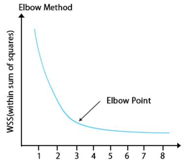
E-commerce industries use K-means clustering to group customers based on their behavioral patterns. Risk Analytics also utilizes K-means clustering for similar purposes.
Below is the Python code:

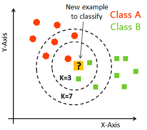
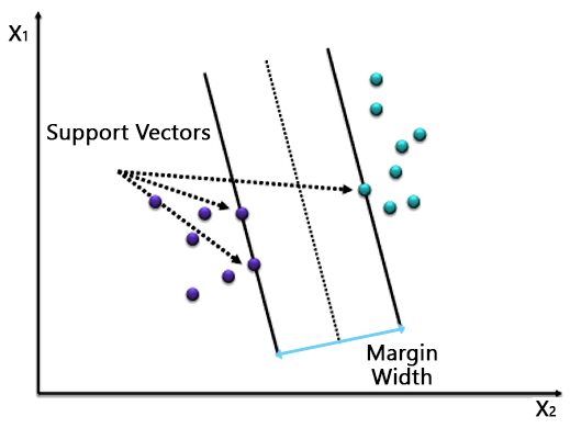
3. K-Nearest neighbors
K-nearest neighbor is the most straightforward of all AI classifiers. However, it varies from other AI procedures in that it doesn’t deliver a model. Instead, it is a straightforward calculation that stores every accessible case and characterizes new examples dependent on a likeness measure.
It works very well when there is a separation between models. However, the learning rate becomes moderate when dealing with a large preparation set and a nontrivial separation calculation.
You can use machine learning algorithms for both classification and regression problems. The idea behind the KNN method is that it predicts the value of a new data point based on its K K-nearest neighbors. People generally prefer using an odd number for K to avoid potential conflicts. When classifying a new data point, they consider the class with the highest mode within the neighbors. For regression problems, they use the mean as the value.
KNN is typically written as
![]()
People use KNN to build a recommendation engine.
4. Principal Components Analysis
On the off chance that you need a higher-dimensional space. You must choose a reason for that space and just the 200 most significant scores of that premise. This base is known as a principal component. The subset you choose creates another space that is smaller in size compared to the original space. It keeps up, however, much of the multifaceted nature of information as could be expected.
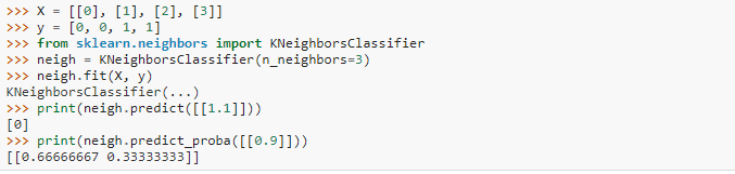
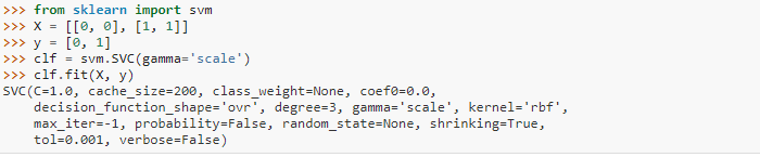
7. Support Vector Machines
A classification algorithm where a hyperplane separates the two classes. In a binary classification problem, we identify two vectors from two distinct classes as the support vectors and draw the hyperplane at a maximum distance from the support vectors.
As you can see, a single line separates the two classes. However, in most cases, the data would not be perfect, and a simple hyperplane would not be able to separate the classes. Hence, it would be best to tune parameters such as Regularization, Kernel, Gamma, etc.
You can choose between a linear or polynomial kernel based on how you want to separate the data. In this case, the kernel is linear. In the case of Regularization, you need to choose an optimum value of C, as a high value could lead to overfitting, while a small value could underfit the model. Gamma defines the influence of a single training example. We consider points close to the line as high gamma and points farther away as low gamma.
In sklearn, SVM is written as:
![]()
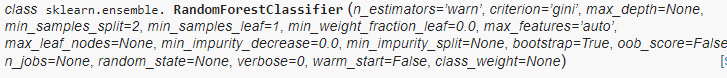
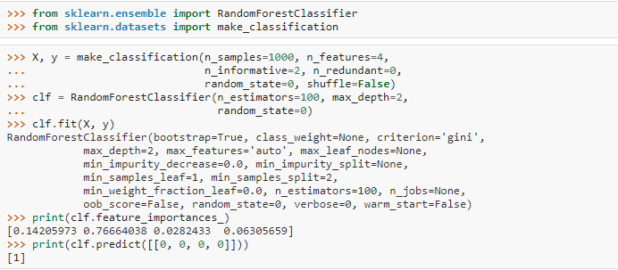
8. Random Forest
We need to reduce the model’s variance to reduce overfitting in Decision Trees. This led to the development of the bagging technique. Bagging involves aggregating the outputs of multiple classifiers to create the final prediction. Random Forest is a specific bagging method that divides the dataset into various subsets through random sampling and selects features randomly for each subset. It then applies the Decision Tree algorithm to these sampled datasets to generate predictions.
In regression problems, we obtain the final prediction by averaging the outputs of all the individual models. In classification problems, we select the class with the highest votes among the individual models to classify the data point. Random Forest is not influenced by outliers or missing values in the data; it also helps in dimensionality reduction. However, it is not interpretable, a drawback for Random Forest.
In Python, you could code Random Forest as:
Conclusion
Data Scientist is the sexiest job in the 21st century, and Machine Learning is certainly one of its key areas of expertise. To be a Data Scientist, one needs to understand all machine learning algorithms and several other new techniques, such as Deep Learning.
Recommended Articles
This has been a guide to Machine Learning Algorithms. Here, we discuss the introduction, importance, and types, along with different algorithms for machine learning. You can also go through our other suggested articles to learn more –
