Excel Interpolate (Table of Contents)
Introduction to Interpolate in Excel
Interpolating in Excel helps you estimate a value between two known values. For example, you have data on the number of social media followers and know the followers count in week 1 and week 3. In that case, you can use interpolation to estimate the followers in week 2.
This kind of forecasting is useful in many kinds of analysis, like investing, establishing strategies, insurance decisions, price movements, stocks, share markets, etc.
Excel has many functions, including “INTERPOLATE,” to help you do this. This article will look at different methods to interpolate in Excel.
Interpolation Methods
1. Simple Mathematics Formula
A simple mathematical formula is a mathematical equation used to represent a relationship between two or more variables. It is a concise and efficient way to describe a mathematical concept or relationship. It can solve problems in various fields, such as science, engineering, finance, and economics.
So, the simple formula for interpolation is:
Where:
- x1 and x2 are the known values of the independent variable that represent the unknown value of x that needs a functional value.
- y1 and y2 are the corresponding values of the dependent variable for x1 and x2, respectively.
- x represents the independent variable value for which we want to estimate the corresponding value of the dependent variable, y.
This formula finds the equation of a straight line passing through the known points (x1, y1) and (x2, y2) and then uses this line to compute the function value at the given value of x. The estimate’s accuracy depends on the degree to which the interpolated function is linear between the known points.
2. FORECAST Function
The FORECAST function estimates a value based on existing values and a linear trend. It is more convenient as it does not require memorizing any formula.
It has the following syntax:
where,
- x: the value whose corresponding value (y) we must predict.
- known_y’s a known range of y values.
- known_x’s: known range of x values..
3. FORECAST Function along with OFFSET and MATCH Function
While the Forecast Function is useful for estimating missing values in data, combining it with the OFFSET and MATCH functions can lead to more accurate results.
The syntax for this function is:
4. FORECAST.LINEAR Function
If you use Office 365, you will have access to the FORECAST.LINEAR function. FORECAST. The LINEAR function can handle multiple independent variables, whereas the Forecast function only works with a single independent variable.
When you use FORECAST, the LINEAR function in Excel assumes that changes in the independent variable (x) can be used to predict changes in the dependent variable (y). This means that if you have a set of known values for both x and y, you can use the function to make predictions about future values of y based on changes in x.
5. TREND Function
The TREND function in Excel helps you find a straight line that fits a set of data points and can even help you predict future values based on that line. Returning an array of y-values corresponding to the x-values can give you a sense of how the data trends over time.
This function is particularly handy for finding missing data points outside the range of your existing data.
The syntax of the TREND function is
6. INTERCEPT Function
The INTERCEPT function in Excel calculates the y-intercept of a linear regression line that includes a set of data points. It gives the y-intercept value where the linear regression line intersects the y-axis.
This function can be really useful when the x-value is missing. Using the available data points, the INTERCEPT function can still accurately estimate where the regression line intersects the y-axis, even if you don’t have a specific value for x.
The syntax for the INTERCEPT function is as follows:
The y-intercept is the point where the regression line crosses the y-axis and represents the value of y when x is zero.
7. XLOOKUP Function
XLOOKUP function allows the search for a value in a particular range and returns a related value from another range. It is similar to the VLOOKUP and HLOOKUP functions but delivers more flexibility. To use XLOOKUP for interpolation, set up your data in two separate ranges, with the x values in one range and the y values in another. Then you could use a formula like LINEST, TREND, or FORECAST to interpolate the missing value.
The syntax for XLOOKUP:
Examples of Interpolate in Excel
After understanding the functions for interpolation, let’s explore how to apply them with the help of some examples.
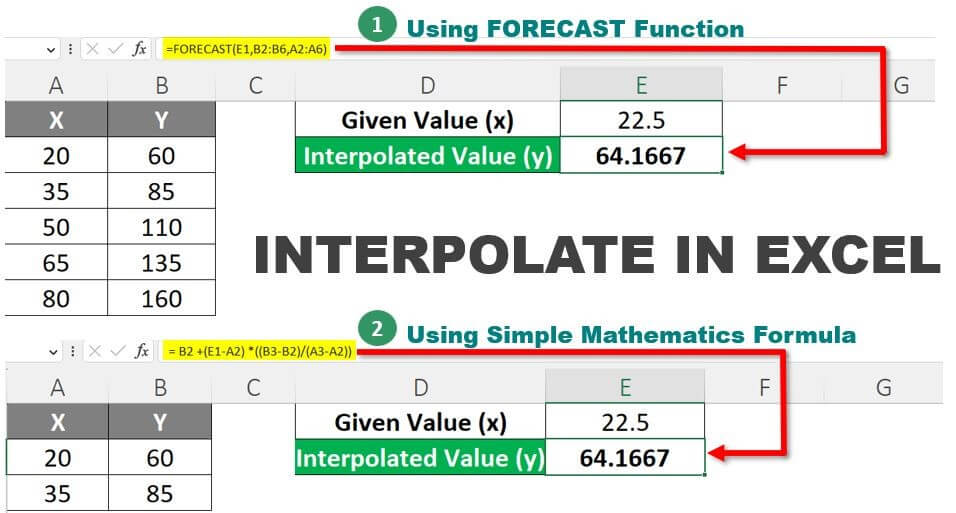
Example #1 Using Simple Mathematics Formula
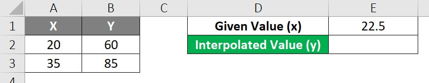
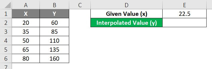
We have a dataset with two known values of x and y. We want to estimate the value of y if x=22.5 using interpolation.
Solution:
Step 1: Select Cell E2
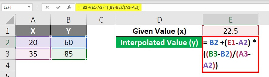
Step 2: We will apply the simple mathematics formula y = y1 + (x – x1) * (y2 – y1) / (x2 – x1) to find the corresponding y-value.
In this example, we will add the following formula in cell E2:
where,
y1 = B2, x = E1, x1 = A2, y2 = B3, y1 = B2, x2 = A3, and x1 = A2.
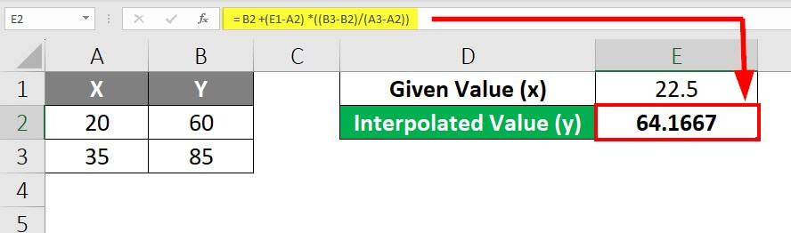
Step 3: Press Enter to get the interpolated y-value.
There can be times when it becomes difficult to memorize the formula. The FORECAST function can be useful in such cases.
Example #2 Using FORECAST Function
Using the Excel Forecast Function, we can interpolate the same value in Example 1.
Solution:
Step 1: Select Cell E2
Step 2: Enter the formula:
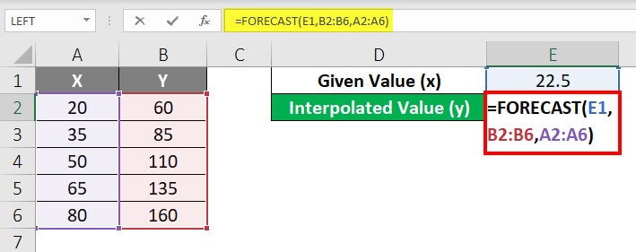
Explanation of formula:
In the formula FORECAST(x, known_y’s, known_x’s), x-value = 22.5 (in cell E1), known y’s = B2:B6, known x’s = A2:A6
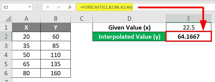
So we can see in the above image that the FORECAST function also works well for this purpose.
Example #3 Using the FORECAST with OFFSET Function
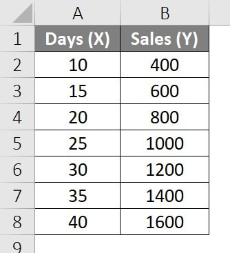
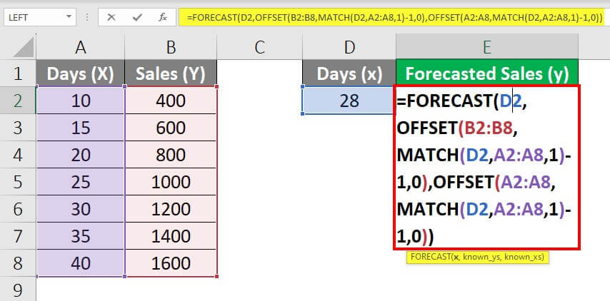
Consider the following dataset for a retail firm displaying the number of units sold daily. The sales values are presented linearly, and we need to estimate the sales for a new period of 28 days. The dataset already contains the sales figures for known periods of 10, 15, 20, 25, 30, 35, and 40 days, so we will use the FORECAST and OFFSET functions together to create an interpolation formula. The objective of the formula is to accurately estimate the sales value for this new period of 28 days by utilizing the known sales data.
Solution:
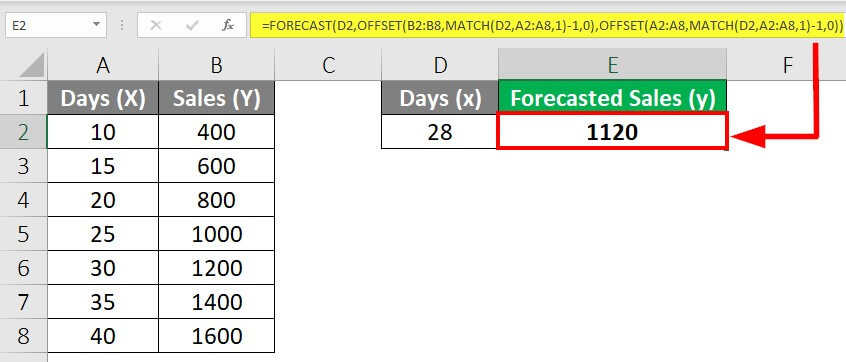
The FORECAST function will perform linear regression on the given data set and predict the sales value for the new period of 28 days based on the relationship between the Days and Sales variables in the data set. The OFFSET function will select the relevant data ranges for the forecast calculation.
Step 1: Locate the x-value, i.e., 28 days in cell D2.
Step 2: Enter the formula in cell E2:
Let us understand how the formula works in this example:
- MATCH(D2, A2:A8, 1)-1: Finds the position of the largest value in the Days column that is less than or equal to the forecasted number of days (D2). The “-1” gets subtracted to adjust because the OFFSET function starts counting from 0.
- OFFSET(B2:B8, MATCH(D2, A2:A8, 1)-1, 0): Selects the Sales values corresponding to the days’ range in the linear regression analysis. The starting point of the range is B2, and the MATCH function determines the number of rows to move down.
- OFFSET(A2:A8, MATCH(D2, A2:A8, 1)-1, 0): Select the Days values corresponding to the days’ range in the linear regression analysis. The starting point of the range is A2, and the MATCH function determines the number of rows to move down.
- FORECAST(D2, OFFSET(B2:B8, MATCH(D2, A2:A8, 1)-1, 0), OFFSET(A2:A8, MATCH(D2, A2:A8, 1)-1, 0)): Takes the forecasted number of days (D2) and the ranges of Sales and Days values selected by the OFFSET functions as arguments to estimate the expected Sales value for the given number of days.
Example #4 Using the Forecast.linear Function
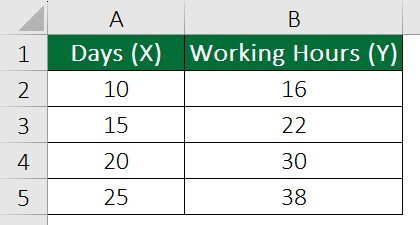
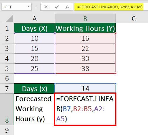
We have a dataset of the graphics department in a publishing company about the working hours of 30 employees over a span of 25 days, with data points available for every 5th day (i.e., on days 10, 15, 20, and 25). To estimate the working hours for any number of days between 1 and 25, we can use FORECAST.LINEAR function to perform the interpolation. For instance, we will apply the function to determine the working hours for 14 days based on the available data points.
Solution:
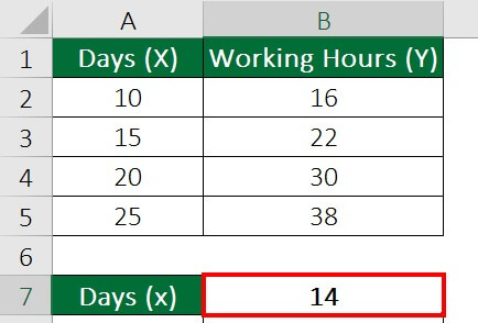
Step 1: To calculate the working hours for 14 days, locate this value in B7.
Step 2: Enter the formula in cell B8:
where,
B7 – x value that can change as per the need.
B2:B5 – the range of working hours, i.e., known y’s
A2:A5 – the range of days, i.e., known x’s
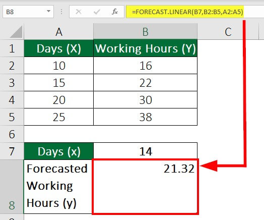
Thus, the working hours for 14 days could be 21.32, i.e., 21 hours, 19 minutes, and 12 seconds.
Similarly, we can find the working hours for any number of days between 1 to 25.
Example #5 Using Trend Function
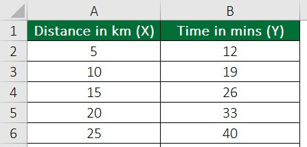
We have a dataset about the distance a vehicle covers in a certain period. The data present shows the time taken for every increasing 5 km. For instance, the vehicle covers a distance of 5 km in 12 mins and 25 km in 40 mins. Using the Trend Function, find the time required for any distance covered beyond 25 km.
Solution:
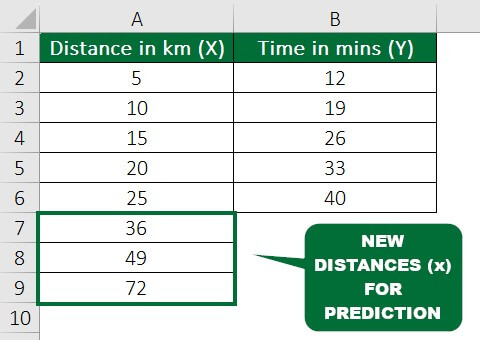
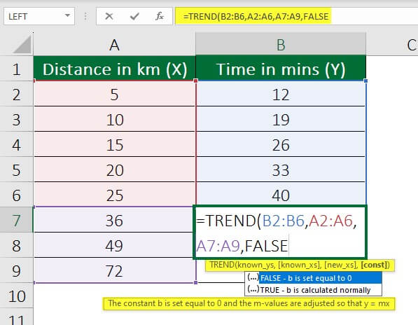
Step 1: Consider 36, 49, and 72 km (the new x’s) as the desired new data from A7:A9.
Step 2: We will input two formulas to apply the Trend Function Formulas in cell B7 with varying fourth arguments.
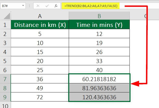
The const argument is set to FALSE in the first formula, =TREND(B2:B6, A2:A6, A7:A9, FALSE). This means the trend will be according to distance (x) from 0 km.
The result of the first formula would be:
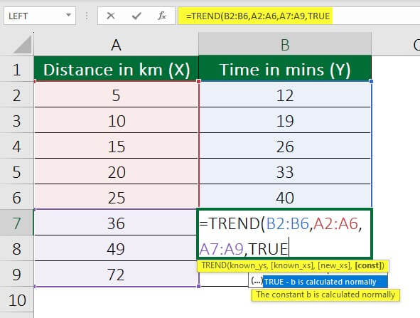
If we don’t want to consider the data from the origin (i.e., 0 KM), we can use the ‘cont’ as TRUE.
This can be beneficial in cases where the data does not naturally pass through the origin, or there is a valid reason to assume that the trendline should not pass through the origin.
Step 3:
We will apply the second formula, =TREND(B2:B6, A2:A6, A7:A9, TRUE), where the const argument is set to TRUE. This means that the y-intercept is not forced to be zero. Thus, Excel will ignore the origin and calculate the value normally per the data.
The result of the second formula would be:
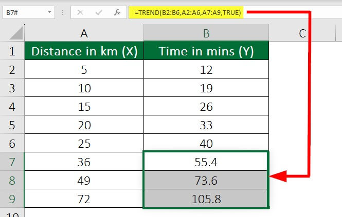
The distance covered will differ depending on the choice of the function.
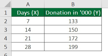
Example #6 Using the Intercept Function
The NGO has collected donations over 28 days and has recorded the amount received at the end of each week. The data shows the number of donations starting from the 7th day. We need to determine if the NGO had any previous donations, i.e., donations on Day 1 (before starting this campaign). Using the Intercept Function, let’s see how we can analyze this.
Solution:
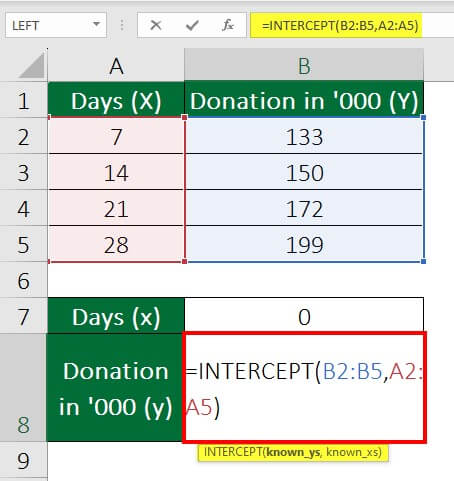
Step 1: Select cell B7 as the location to perform the function.
Step 2: Enter the formula in cell B7:
Step 3: Press Enter after selecting the y’s and x’s range.
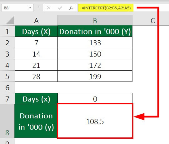
Hence, the amount of donations before starting this charity campaign, i.e., on Day 1, is $108500.
The INTERCEPT Function considers a linear relationship between the Days and Donation ($) and calculates the y-intercept suitable considering the x-value as 0.
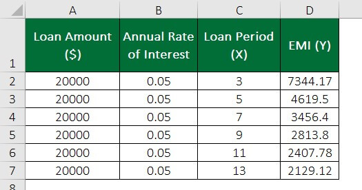
Example #7 Using the XLOOKUP Function
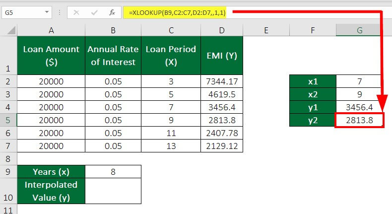
We have the structure of equated monthly installments (EMI) for a loan of $20000 at a 5% interest rate for a combination of years. The task is to find the EMI options for the desired years (x-coordinate) using XLOOKUP and FORECAST functions.
Solution:
We need to determine the values of x1, x2, y1, and y2 for a desired x-value.
Step 1: Locate the x-coordinate in cell B9 and the values we need to find can be in cells G2 to G5.
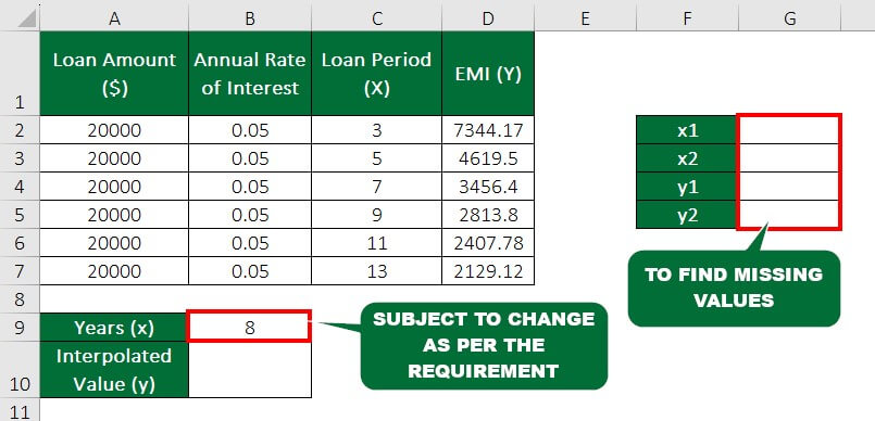
We will have 8 as the x-coordinate, which can differ per the user’s requirements.
Step 2: Now, to find the value for x1, enter the following formula in cell G2 –
=XLOOKUP(B9,C2:C7,C2:C7,,-1,1)
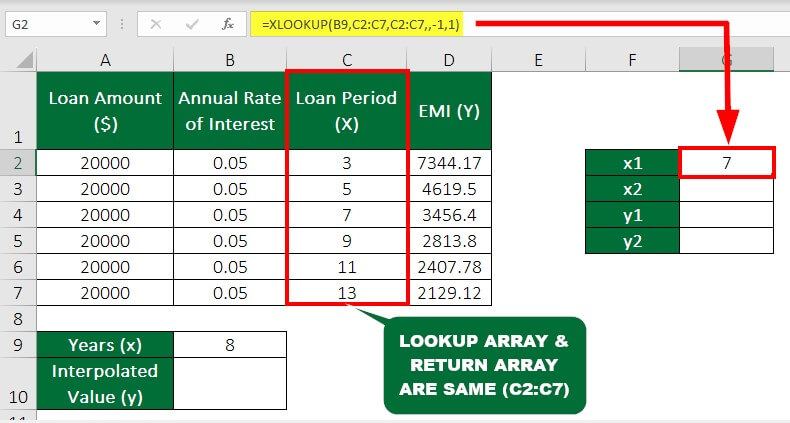
Here, the lookup and return array is the same as we are looking for x1. -1 as match_mode refers to searching for an exact match or a smaller value in the range.
We receive the value of x1 as 7 in cell G2.
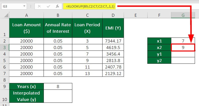
Step 3: Similarly, we calculate x2 in cell B3 by taking the match_mode as 1 to find the exact match or the next higher value in the range.
Therefore, the formula will be
=XLOOKUP(B9,C2:C7,C2:C7,,1,1)
Excel will give the value of x2 as 9.
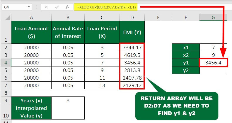
Step 4: Change the return_array to C2:C7 to determine y1 and y2 in cells G4 and G5 per the images below.
Therefore, the formulas will be
y1 =XLOOKUP(B9,C2:C7,D2:D7,,-1,1)
y2 =XLOOKUP(B9,C2:C7,D2:D7,,1,1)
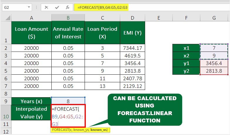
Now that we know the required values, we can determine the y-intercept, i.e., Interpolated Value of Loan Amount for 8 years, using the Forecast Function.
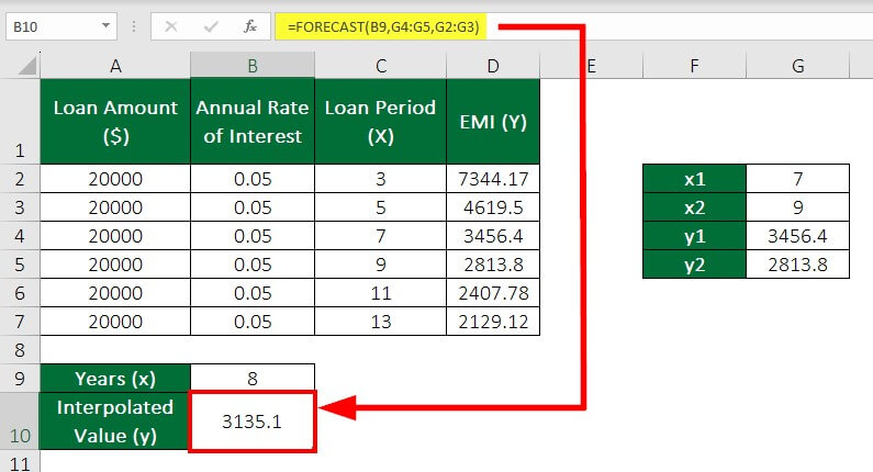
Step 5: Enter the Forecast Function formula in cell B10
Things to Remember About Interpolate in Excel
- Linear Interpolation is not an accurate method in MS Excel; however, it is time-saving and fast.
- Linear Interpolation can even predict values for rainfall, geographical data points, etc.
- If the data is not linear, other methods that can be useful for interpolation are Polynomial Interpolation, Spline Interpolation, etc.
- The FORECAST function can extrapolate or predict future values.
Frequently Asked Questions
Q1. What are Interpolation and Extrapolation in Excel?
Answer:
|
Aspect |
Interpolation |
Extrapolation |
| Definition | Interpolation estimates the value for missing data from a given range | Extrapolation estimates the value for missing data outside a given range |
| Data Relation | A smooth and continuous relationship between known data figures | A continuation of the same pattern outside the given known data |
| Risk | Less risky as it involves known data points | Riskier as it involves a value outside the known data range |
| Excel Functions To Calculate |
|
Excel does not offer any specific function for extrapolation. Some users may choose TREND or FORECAST, which could be complex without actual data. |
| Example | Estimating the temperature at 3 pm from the given temperatures at 2 pm and 4 pm | Estimating the temperature at 7 pm considering the given temperatures from 2 pm to 4 pm |
Q2. What are the Uses of Data Interpolation?
Answer:
Missing Data: Interpolation can estimate missing data points in a dataset.
Smoothing Data: Interpolation can also smooth out noisy data by filling in gaps between known data points. It can reduce the impact of outliers or noise in the data.
Future Value Predictions: Interpolation can predict future values of a variable using the known data points.
Continuous Curves: Interpolation can create continuous curves or surfaces from scattered data points in computer graphics to create smooth animations.
Derivatives and Integrals: Interpolation can calculate the derivatives and integrals of a function if a function is not available in an explicit form.
Measurement and Adjustment: Interpolation can calculate and adjust instruments using known data points.
Q3. What is the Importance of Interpolation in Numerical Analysis?
Answer: Interpolation is crucial in scientific computing, engineering, and many other fields where accurate data modeling and prediction are important. Interpolation allows:
- Creation of continuous functions that can predict values between known data points.
- Data analysis, signal processing, and image processing for data smoothing and filtering.
- Development of numerical methods for solving differential equations, optimization problems, and other mathematical models.
- Construction of mathematical models for physical systems, such as weather forecasting, oceanography, and the study of material properties.
- Data visualization for the creation of smooth curves and surfaces that can represent complex data sets.
- Machine learning algorithms, where interpolation predicts missing values and creates accurate models of complex systems.
- Development of mathematical models for financial analysis, such as pricing derivative securities and estimating risk.
- Scientific research for comparing and analyzing complex data sets and helping researchers to make predictions and test hypotheses.
Note: If you are aiming to master tools like Excel, there are numerous courses and certifications available to help you achieve that goal. Alongside Microsoft certifications, there are various other IT certifications that you can use to demonstrate your skills. To do well you need to work through practice exam questions and use resources like Microsoft AZ-500 Exam Dumps improve your preparation. If you don’t need a formal certification, there are lots of training companies that offer Excel courses like this one in London that has good reviews.
Recommended Articles
This is a guide to Interpolate in Excel. Here, we discuss how to interpolate in Excel using functions like FORECAST, LINEAR, TREND, and more. TREND Function. You can also go through our other suggested articles:
