Updated May 4, 2023
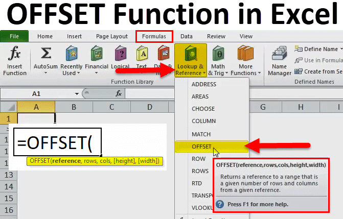
What is OFFSET Function in Excel
The offset function helps to get the value stored in a selected row or column or array of a row-column matrix by calling out the row and column number concerning the cell value. The offset function starts counting the row and column number once we fix the reference cell, and that cell will become its first point to start counting.
Syntax
Below is the OFFSET Syntax in Excel:
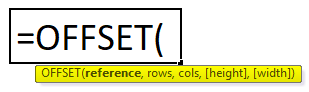
OFFSET Function in Excel consists of the following arguments:
- Reference: It is the argument on which we want to base the offset. It could be a cell reference or a range of adjacent cells; if not, Offset returns the #VALUE! Error value.
- Rows: It is the no. of rows to offset. If we use a positive number, it offsets the rows below; if a negative number is used, it offsets the above.
- Columns: It is for no. of columns to offset. So, it is the same concept as Rows; if we use a positive number, it offsets the columns to the right, and if a negative number is used, it offsets the columns on the left.
- Height: This argument is optional. It should be a positive number. It is a number that represents the number of rows in the returned reference.
- Width: This is also an optional argument. It must be a positive number. It is a number that represents the number of columns in the returned reference.
Notes:
- The OFFSET Function in Excel returns the #REF! Error value if rows and columns offset reference over the edge of the worksheet.
- The OFFSET function is supposed to be the same height or width as a reference if height or width is omitted.
- OFFSET returns a reference; it does not move any cells or range of cells or change the selection. It can be used with any function expecting a reference argument.
How to Use the OFFSET Function in Excel?
OFFSET Function in Excel is straightforward to use. Let us understand the working of the OFFSET Function in Excel by some OFFSET Formula examples.
Example #1
The Offset formula returns a cell reference based on a starting point, rows, and columns that we specify. We can see it in the given below example:
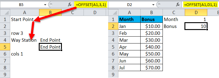
=OFFSET (A1, 3, 1)
The formula tells Excel to consider cell A1 for starting point (reference), then move three rows down (rows) and 1 column to the left (columns argument). After this, the OFFSET formula returns the value in cell B4.
The picture on the left shows the route of the function, and the screenshot on the right demonstrates how we can use the OFFSET formula in real time. The difference between the two formulas is that the second (on the right) includes a cell reference (D1) in the row’s argument. But since cell D1 contains number 1, and the same number appears in the rows argument of the first formula, both would return an identical result – the value in B2.
Example #2
The OFFSET Function can also be used with the other Excel function; hence, we will see the SUM Function in this example.
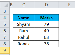
In the above picture, suppose we have to find out the number of marks, then we can also use the OFFSET function.
The formula is below:
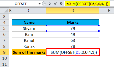
So, in the above formula, D5 is the first cell where the data begins, which is a reference as starting cell. After that, the rows and column value is 0, so we can put it as 0,0. Then there is 4, which means four rows below the reference for which Excel needs to calculate the sum, and then, at last, it is 1, which means there is 1 column as width.
We can refer to the above pic to co-relate the explained example.
And below is the result:
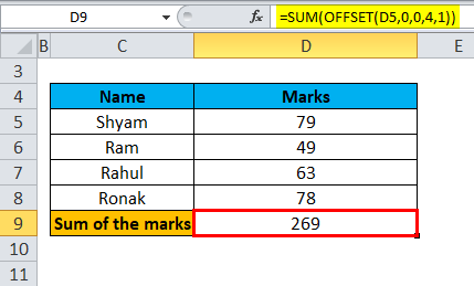
We have to press Enter after entering a formula in the required cell, and then we have the result.
Things to Remember
- The OFFSET Function in Excel returns a reference; it does not move any cells or range of cells.
- If the OFFSET Formula returns a range of cells, the rows and columns always refer to the upper-left cell in the returned range.
- The reference should include a cell or range of cells; otherwise, the formula will return the #VALUE error.
- If the rows and columns are specified over the edge of the spreadsheet, the Offset formula in Excel will return the #REF! Error.
- OFFSET function can be used within any other Excel function which accepts a cell or range reference in its arguments.
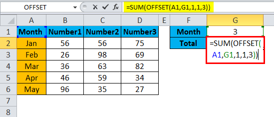
For example, if we use the formula = OFFSET (A1, 3, 1, 1, 3) on its own, it will give a #VALUE! Error, since a range of returns (1 row, three columns) does not fit in a cell. However, if we collate it into the SUM function like below:
=SUM (OFFSET (A1, 3, 1, 1, 3))
The Offset formula returns the sum of values in a 1-row by a 3-column range of three rows below and 1 column to the right of cell A1, i.e., the total values in cells B4:D4.
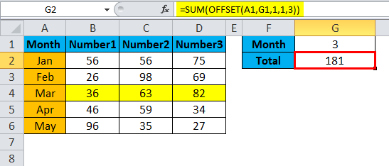
As we can see, 36+63+82 of highlighted Mar equals 181, resulting in G2 after applying the sum and Offset formula. (highlighted in yellow)
Use of OFFSET Function in Excel
As we have seen what the OFFSET function does with the help of the above example, we may have questions Why bother to use the OFFSET formula that is a bit complex? Why not simply use a direct reference like sum or B4:D4?
The OFFSET function in Excel is perfect for below:
- Getting the range from the starting cell: Sometimes, we do not know the exact or actual address of the range; we only know where it starts from a particular cell. In this case, we can use the OFFSET Function, which is easy.
- Creating Dynamic Range: The references like the above example B1:C4 are static, which means they always refer to a given or fixed range. But in some cases, the tasks are easier to perform with dynamic ranges. It especially helps when we work with changing data. For example, we could have a spreadsheet where a new row or column is inserted or added every day/week/month; in this case, the OFFSET function will help.
Limitations and Alternatives of the OFFSET Function in Excel
As every formula in Excel has limitations and alternatives, we have seen how and when to use the OFFSET Function in Excel.
Below are the critical limitations of the OFFSET function in Excel:
- Resource-hungry Function: The formula will be recalculated for the entire set whenever there is a change in the source data, which keeps Excel busy for a longer time. A small spreadsheet will not affect that much, but Excel may take time to recalculate if there are many spreadsheets.
- Difficulty in review: As we know, the references returned by the Offset function are dynamic or changing and may contain a big formula, which may find tricky to correct or edit as per requirement.
Alternatives of the OFFSET Function in Excel:
- INDEX function: The INDEX function in Excel may also create a dynamic range of references. It is not the same as OFFSET. But like OFFSET, the INDEX function is not that volatile; hence it won’t slow down Excel, which is a limitation for OFFSET.
- INDIRECT Function: We can also use the INDIRECT function to create a dynamic range of references from many sources like cell values, text, and the named ranges.
Recommended Articles
This has been a guide to OFFSET in Excel. Here we discuss the OFFSET Formula in Excel and How to use the OFFSET Function in Excel, along with practical examples and a downloadable Excel template. You can also go through our other suggested articles –
