Introduction to Split Cell in Excel

Split Cell in Excel means dividing a single cell’s data into multiple cells. It can be super useful when data from multiple columns or rows are included in a single cell. Splitting allows you to analyze and present the information more organized and meaningfully.

There are different ways to split cells in Excel, depending on what you want to achieve.

If you want to save time, then use a keyboard shortcut. You can select the data and press ALT + A + E keys to split cells simultaneously. You can also split a cell in Excel with fixed width if you want a specific length to break or use delimiters with special characters like commas, semicolons, spaces, etc.

In this article, we will learn various methods to split cells in Excel using different examples.

Example #1

You can download this Split Cell Excel Template here – Split Cell Excel Template

Split Merged Cells in Excel

This is the simplest method of splitting or Unmerging cells in Excel.

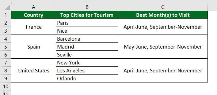
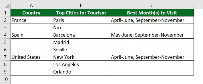
Consider the below data of tourist places of a particular country and their best month to visit. We want to split the already merged cells (columns A and C).

Solution:
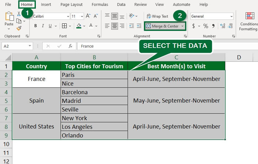
Step 1: Select the entire data.
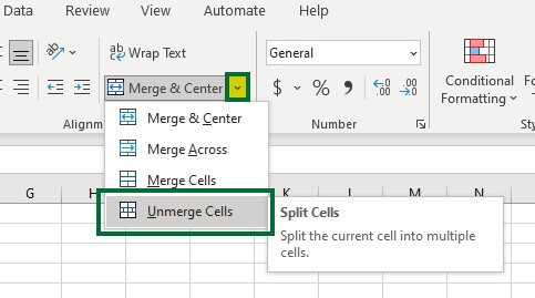
Step 2: Go to the “Home” tab > Alignment group, and click “Merge & Center“, as shown below.

Note: There is another method. Click the “Dropdown menu” under the “Alignment” group of the “Home” tab. Click on the “Unmerge Cells” option, as shown in the below screenshot.

Result: All merged cells are split successfully, as seen below.

Note: Each merged cell’s content will be displayed on the upper-left cell, and all other merged cells will be empty.

Example #2

Split a Cell Diagonally in Excel

Splitting a cell diagonally adds two labels/heading to a single cell in Excel. This allows you to give heading one for the data in the rows and another for the data in the columns separately, making it easier to read and understand your spreadsheet.

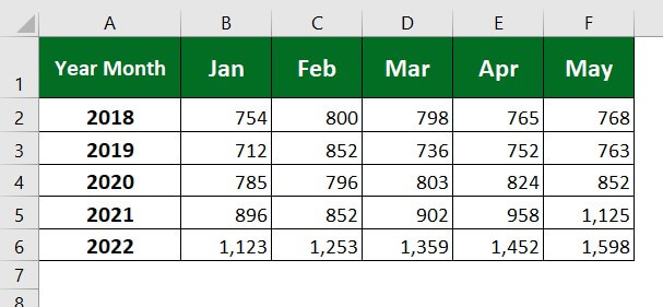
Let’s consider the below sales data of a company. Here, we want to add headings for rows and columns. For better understanding, we will use “Year” for rows and “Month” for columns.

Solution:
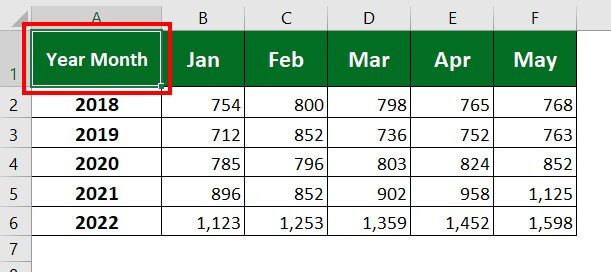
Step 1: Click on “Cell A1″.

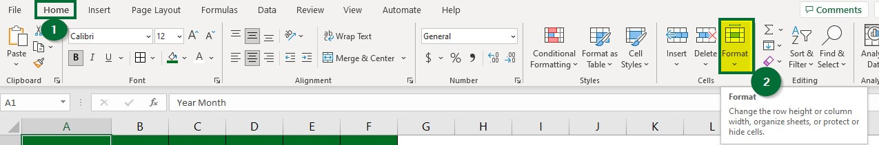
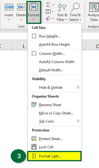
Step 2: Go to the “Home” tab and click on “Format” under the “Cells” group, as shown below.

Step 3: Select “Format Cells” from the Format dropdown window.

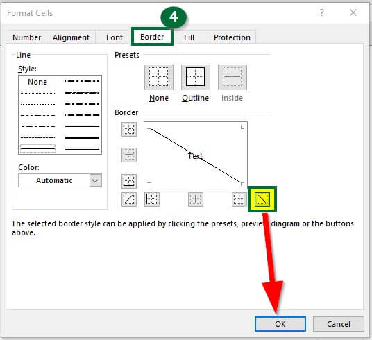
A Format Cells dialog box will appear.

Step 4: Go to the “Border” tab. Click the right side box spitted diagonally as shown below and press “Ok“.

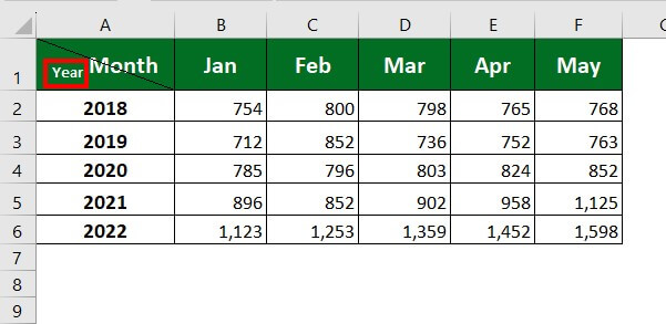
Note: The” Border” preview section will display how the selected diagonal will appear. In the “Format Cells” dialogue box, you can apply multiple formatting per your demand to the selected cell.

The cell is divided diagonally, as shown in the below image.

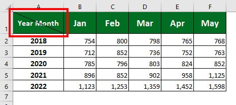
We want to separate the heading (Year and Month) across the diagonal line.

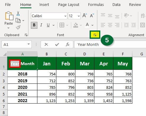
Step 5: Select “Year” and click on the downward arrow at the bottom-right corner of the “Font” group of the “Home” tab.

A Format cells dialog box will appear.

Step 6: Select “Subscript” under the “Effects” section and click on “OK”.

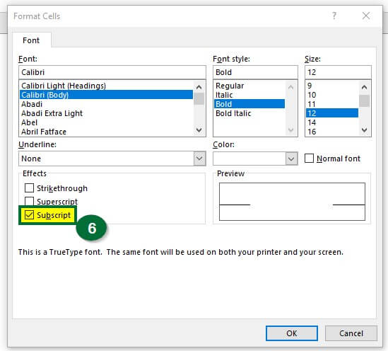
“Year” appears at the bottom of the cell, as shown below.

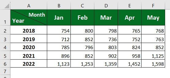
Step 7: Repeat Steps 5 & 6 for “Month” and select “Superscript”.

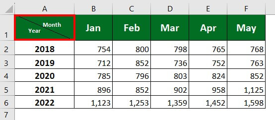
“Month” appears at the top of the cell, as shown above. Now, Adjust the font size and alignment of “Year” and “Month“.

Result: Cell A1 is diagonally separated with “Year” representing rows and “Month” representing Columns.

Example #3

Split Cell in Excel Using Power Query

We can also split cells in Excel using Power Query. In a power query, a column’s data can be split into numerous columns per the requirement. We can split our data by delimiters, positions, numbers of characters, digit-to-non-digits, etc.

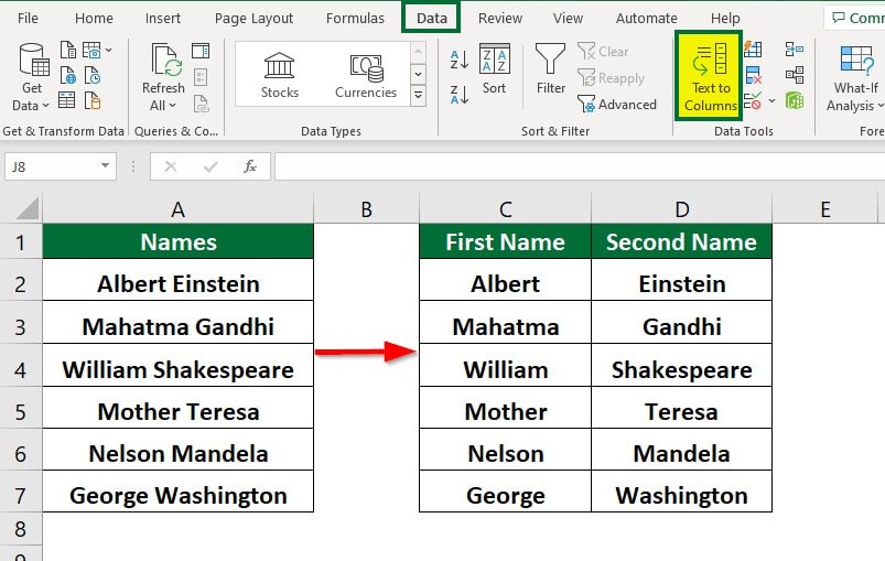
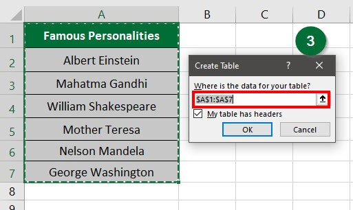
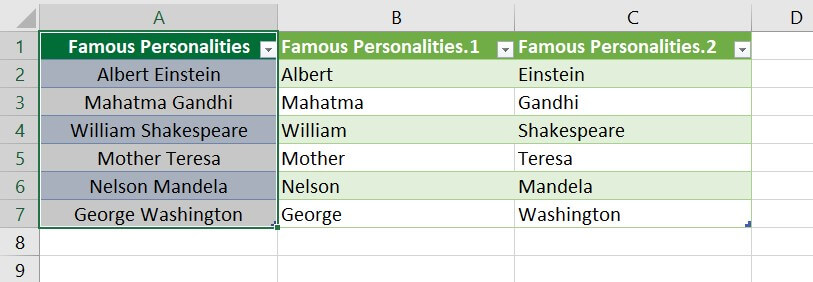
Consider the below data of famous personalities. Here, we want to separate the first and last names into two columns. We will use the delimiter option to split the data.

Solution:
Step 1: Select the entire data range (A2:A7)
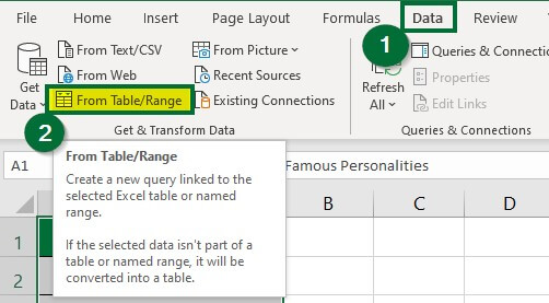
Step 2: Go to the “Data” tab, and click the “From Table/Range” button under the “Get & Transform Data” group.

A “Create Table” dialog box will open.

Step 3: Select the table range and press OK, as shown below.

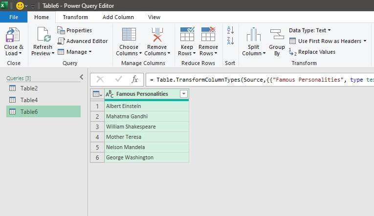
A new window of “Power Query Editor” will open immediately. This editor page will show a preview of our data.

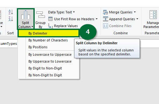
Step 4: Select the entire column and go to the “Home” tab >under “Transform group”> “Split Column”> select “By Delimiter”

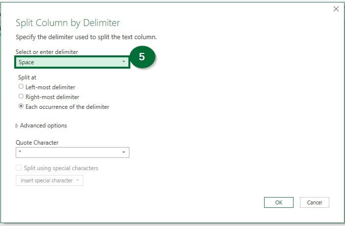
The Split Column By Delimiter window will pop up.
Step 5: Select Space and press OK, as shown below.

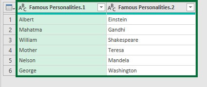
Note: The first name and last name of the original data are separated by space.

The original name is split into two columns in Power Query.

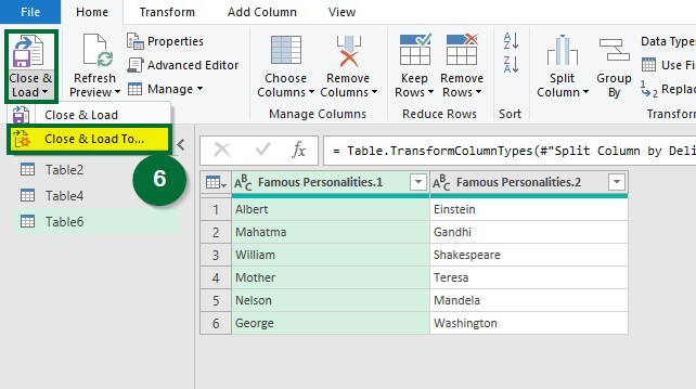
Step 6: Go to “Close & Load” and select “Close & Load To“, as shown below.

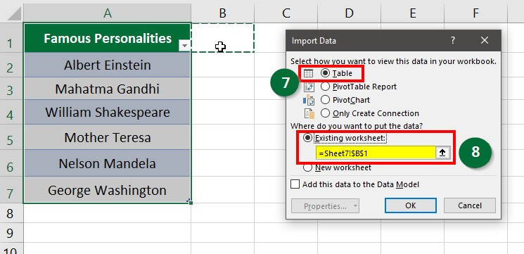
A dialog box named Import Data will open.

Step 7: Select the “Table” option under “Select how you want to view this data in your workbook” and enter the desired cell where we want the data to display in the “Existing workbook”. Click on “OK”.

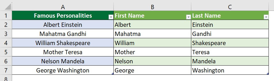
The data from the Power Query Editor will be imported into the desired cell in the original Excel sheet. Refer to the below screenshot.

Step 8: Change the column heading to “First Name” and “Last Name”.

Result: The first name and last name is separated using the power query.

Example #4

Split Cell Using Text-to-Column Function

We can also Split Cell in Excel using the text-to-column Function. Text to Columns function in Excel separates text strings by a specific delimiter such as comma, semicolon, space, and fixed character count.

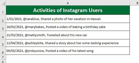
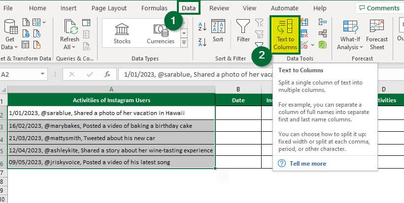
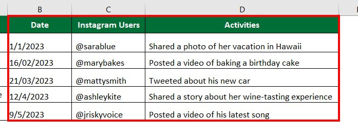
Consider the below data on the activities of Instagram users. Here, all the data is in the same column. We want to separate the data into different columns like Date, Instagram Users, and Activities using the text-to-column delimited method, which involves using a specific character (in this case, a comma) to separate the data into its respective columns.

Solution:
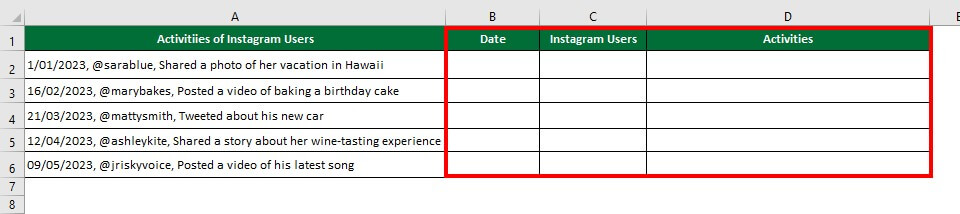
Step 1: Insert three columns as shown in the below image.

Step 2: Select the range “A2:A6″ and Go to the “Data” tab > click “Text to Columns” under the “Data Tools” group, as shown below.

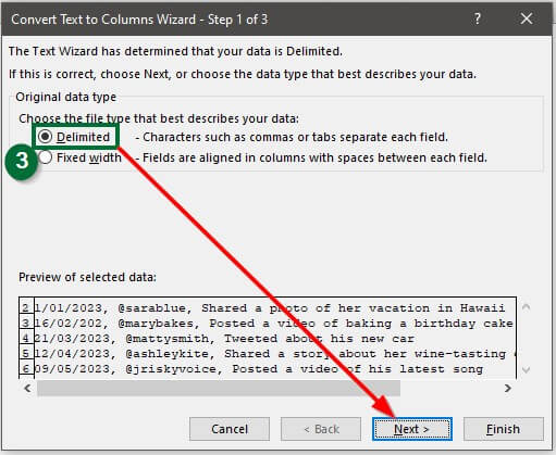
A “Convert Text to Columns Wizard” will open.

Step 3: Select “Delimited” under the “Original data type” and click “Next“.

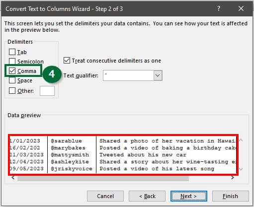
Step 4: Select “Comma” under the “Delimiters” section and click on “Next“.

We can see how the data is separated under the “Data Preview” section.

Step 5: Select “General” and the “Destination” cell. After selecting the destination cell, click on “Finish“.

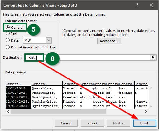
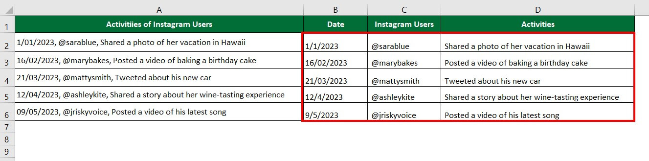
The output is displayed below in three separate columns.

Result: The data of column A is separated into three columns, as shown below.

Example #5

Split Cell in Excel Using Flash Fill

Another method to Split Cells in Excel is by Flash Fill. Flash Fill automatically populates cells with desired data. The Flash Fill method is easy to use and quickly splits data into multiple columns.

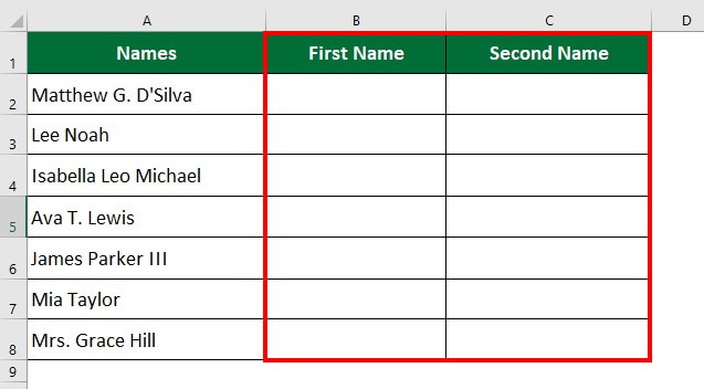
Let’s learn from the below example. We want to split the first and second names using Flash Fill in the data below.

Solution:
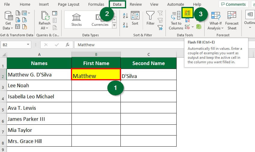
Step 1: Insert two new columns next to the original data and name the column as shown below.

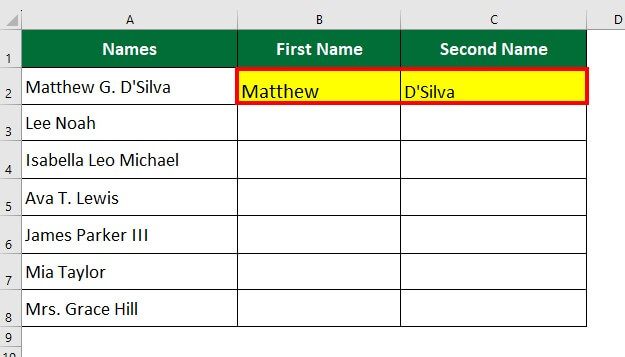
Step 2: Split the content of Cell A2 into Cell B2 and C2. Like, type/enter the first and second names of the original name in the respective cells as seen below.

Step 3: Select “Cell B2″ and Go to the “Data” tab. Click on the “Flash Fill” symbol under the “Data Tools” section.

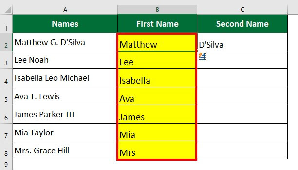
Flash Fill will automatically populate similar data (first name) into other cells. The entire column of B displays the first name of the original names.

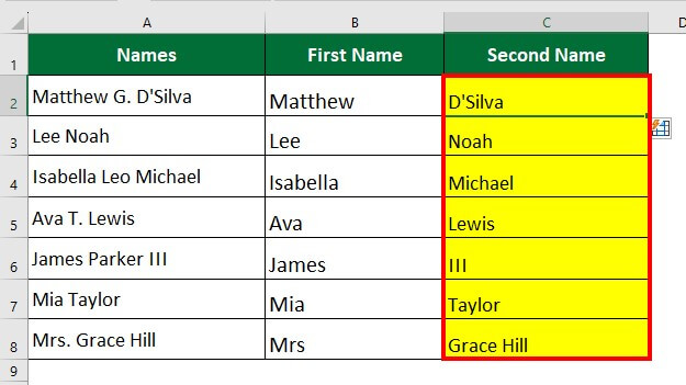
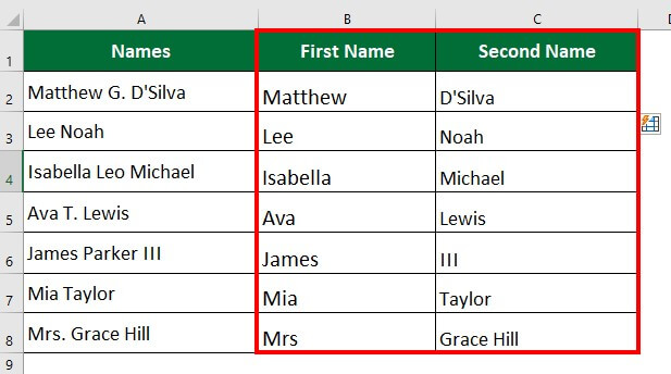
Note: Flash Fill only works when it recognizes a pattern or an example. Always enter a pattern or examples of the output you want. If you do not insert any value in the cell and use click on Flash Fill, It will show an error.

Step 4: Repeat steps 3 on Cell C2 or select cell C2 and press “Ctrl + E“.

Note: The keyboard shortcut for Flash Fill is “Ctrl + E“.

Result: The first and second names are split successfully.

Example #6

Split Cell in Excel Using Text Functions

Although Flash Fill is easy to use, the results are not dynamic. It does not automatically update the output if the source data is changed. Thus to Split Cell in Excel, we can use various Text functions or create formulas to fetch results if we want dynamic results.

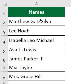
Let’s take the previous example to split full names into first, middle, and last names using LEFT, MID and RIGHT functions.

Solution:

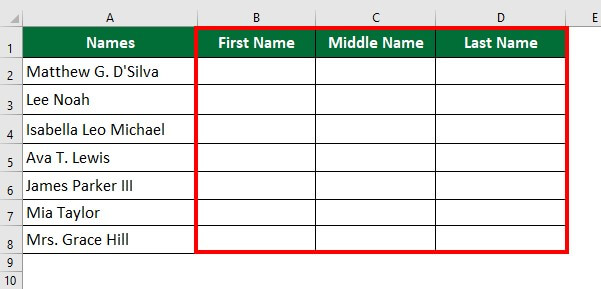
Step 1: Insert three new columns after the original data, as shown below.

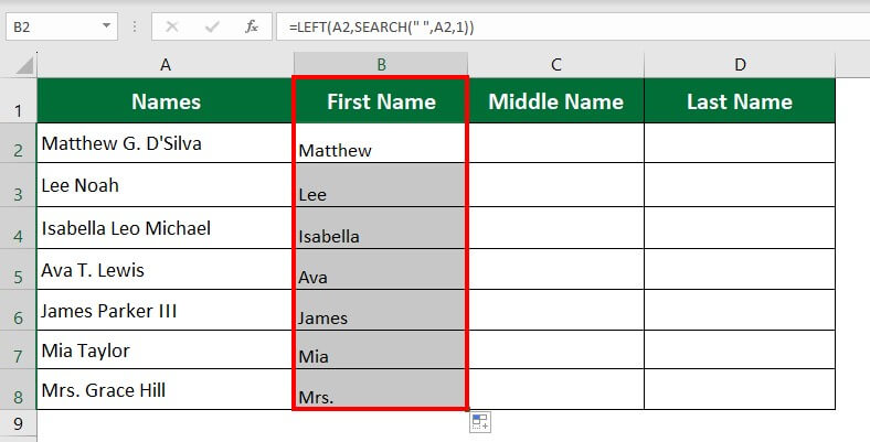
Step 2: Click on Cell B2 and enter the formula “=LEFT(A2,SEARCH(“ “,A2,1))”.

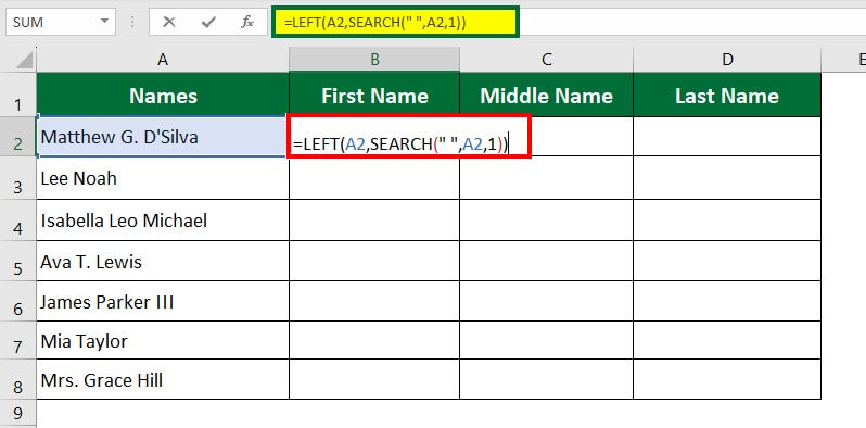
The formula returns the first name, as shown below.

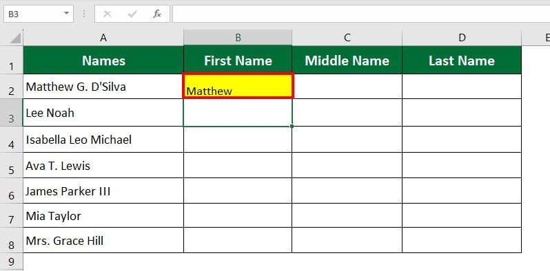
Step 3: Now, select cell B2 and drag it down.

The result is displayed below.

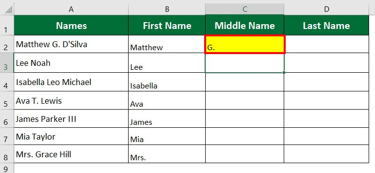
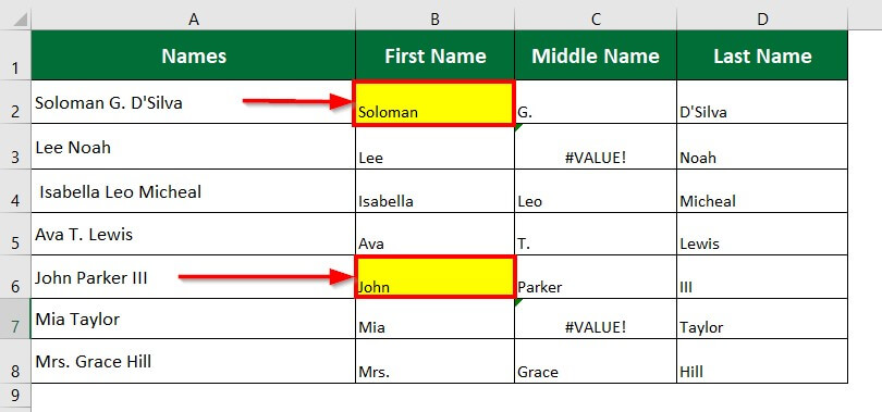
Step 4: Select cell C2 and enter the formula “=MID(A2,SEARCH(“ “,A2)+1,SEARCH(“ “,A2,SEARCH(“ “,A2)+1)-SEARCH(“ “,A2)-1”

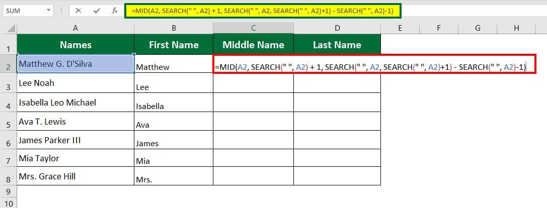
The formula returns the middle name, as shown below.

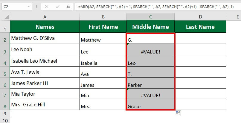
Step 5: Now, drag the cell downward.

Note: The formula will display “#VALUE1″ if the original data contains no middle name.

Step 6: Select Cell D2 and enter the formula “=RIGHT(A2,LEN(A2)-FIND(“*”,SUBSTITUTE(A2,” “,”*”,LEN(A2)-LEN(SUBSTITUTE(A2,” “,””)))))

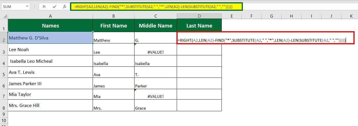
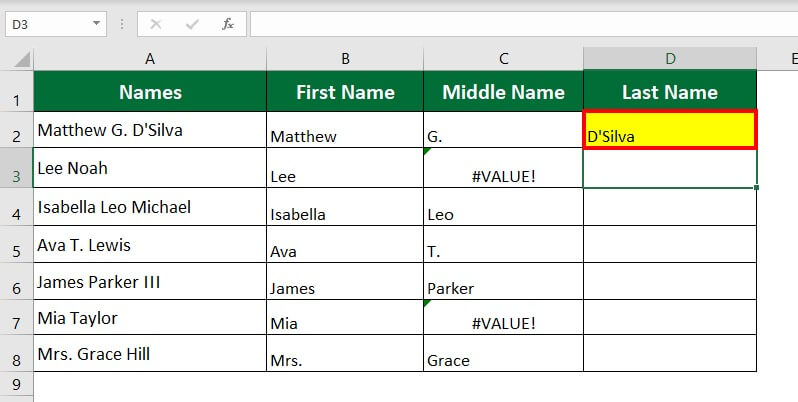
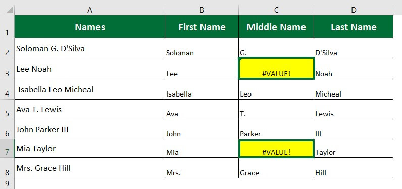
The formula returns the last value in Cell D2, as shown below.

Step 7: Drag Cell D2 downwards. You will get the below result.

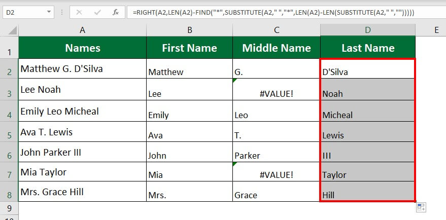
Result: Using text functions, we have successfully separated the first, middle, and last names.

Note: Spilt Cell in Excel using the Text function is dynamic means if the value of the original data is changed, it will automatically get reflected in the output. For example, we have changed Matthew in Cell A2 to Soloman and James to John in Cell A6. The function automatically altered the value of Cell B2 to Soloman and Cell B6 to John, as shown below.

Now, let us learn how to remove “#VALUE!”.

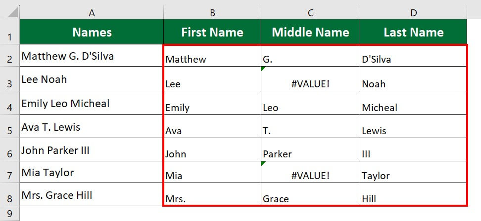
Step 8: Select column 2 (C2:C8) and enter the formula “=IFERROR(MID(A3, SEARCH(” “, A3) + 1, SEARCH(” “, A3, SEARCH(” “, A3)+1) – SEARCH(” “, A3)-1),””)”

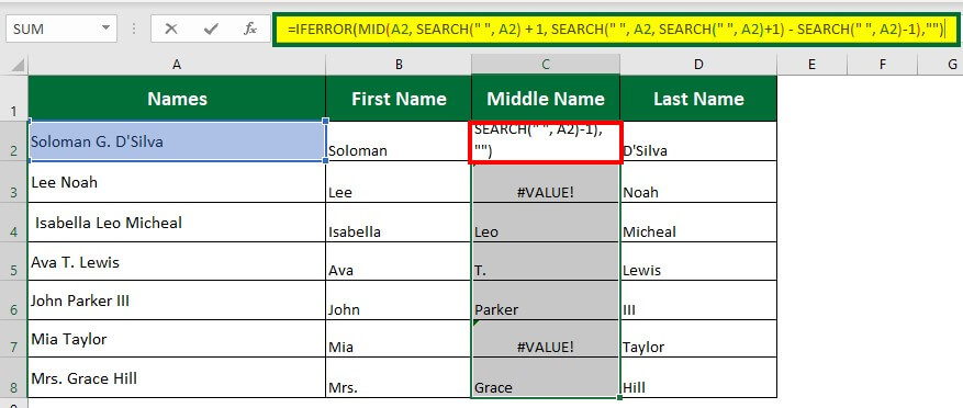
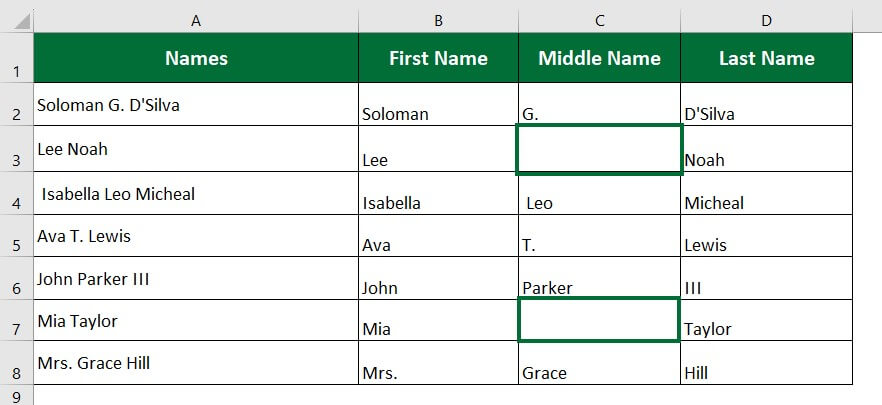
Step 9: Press “Enter“.

Result: The cells which show “#VALUE!” will be blank.

Things to Remember

The keyboard shortcut for unmerging cells is “Alt + H+ M + U“.
The shortcut for flash fill is “Ctrl+ E“. The result from Flash Fill is static.
The keyboard shortcut for “Format Cells” is “CTRL + 1“, or select the cell you want to format and right-click from the mouse and choose “Format Cells”.
The text functions in Excel are dynamic, which means if you change the values of the original data, it will automatically get reflected in the result.

Frequently Asked Questions(FAQs)

Q1. What are Split Cells in Excel?
Answer: Split Cell in Excel is a feature to split or divide the content of single cells into numerous cells depending upon the task. For example, split cells are useful in separating first and last names.

Q2. How do split cells extract data in Excel?
Answer: There are various methods to Split Cell in Excel to extract data which are as follows:

Method	Description
Power Query	Splits a column’s data into multiple columns based on delimiters, positions, characters, etc.
Text to Columns	Splits the contents of a cell into two or more columns based on comma, semicolon, space, and fixed character count.
Text Functions	Uses functions like MID, RIGHT, and LEFT for dynamic results.
Flash Fill	Automatically splits strings into cells in the simplest way.

Q3. What is the difference between merge cells and split cells?
Answer: Merging of cells is joining two or more cells into a single cell. In contrast, splitting is the opposite of merging. Splitting cells means separating or dividing one cell content into two or more cells.

Quiz Result
Total Questions	Correct Answers	Wrong Answers	Percentage