Updated July 3, 2023
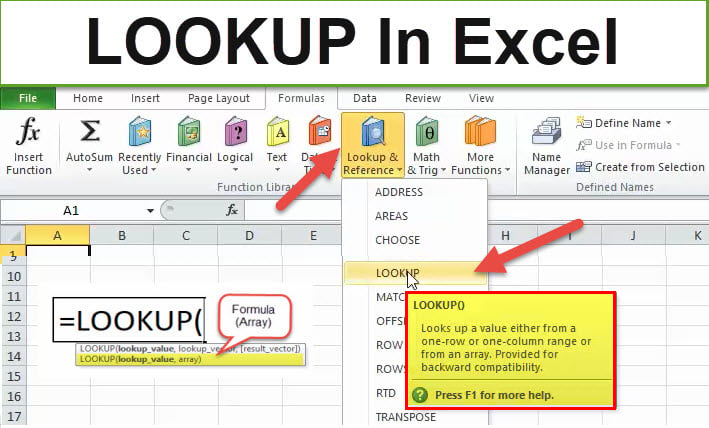
Introduction to LOOKUP Function in Excel
The Lookup function in Excel finds a specific value in a table or spreadsheet and shows you the related information in its adjacent cells in the same row.
For example, if you want to search for the number 5 in a table, you could use the Lookup function to return the other information in the same row or column as 5. The LOOKUP function is a built-in worksheet function in Microsoft Excel. It is available in Lookup & References under the Formula tab.
Syntax of Excel LOOKUP Function, The LOOKUP function in Excel is of two types: Vector and Array.
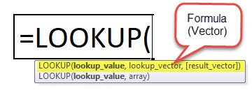
1. Vector form LOOKUP in Excel
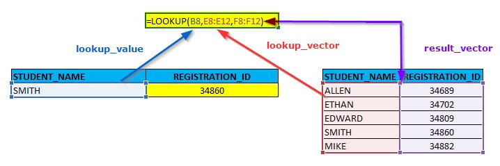
The vector form of the LOOKUP function is useful for searching for a specific value in one row or column and returning a value from the same location in another row or column. For instance, you have a list of students with their names in one column and grades in another, and you want to find a grade for a particular student. The vector form of the LOOKUP function in Excel will search the student’s name and then display their grade from the same row.
If you know the row or column range where the search value is present, you can use this form of the LOOKUP function to get the value from that row or column.
- Lookup Value: (Required) It is the value that we want to search in one row or one column. It can be a text, number, cell reference, value, or name.
- Lookup Vector: (Required) The range of one row or column where the lookup_value will be first searched. The value can be numbers, text, or reference values.
- Result Vector: (Optional) It is the range of a single row or column from where we want to fetch the required value. The size of the result_vector must be the same as that of the lookup vector.
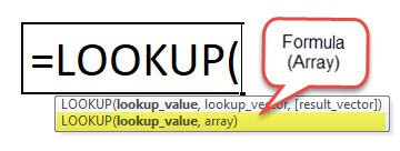
2. Array form LOOKUP in Excel
An array is a combination of values in rows and columns in the form of a table. The array form of the LOOKUP function searches for a specific value in the first row or column and returns a value from the same region in the last row or column of the array. Use this array form only when the values you want to search are in the array’s first row or column.
- Lookup _value: (Required) lookup_value in array form is the value the LOOKUP function searches for in an array.
- Array: (Required)It is the range of cells of multiple rows and columns, like a two-dimensional data (table), where you want to search the lookup_value.
Let’s Learn the Use of the LOOKUP Function in Excel.
In the following section, you will learn how to use the Lookup function with the help of various examples. You will also learn to create a LOOKUP formula to find a value for specific criteria.
Example #1
How to search for a value in a one-column range?
In this example, you will learn how to search for a specific value in one column range using the vector form of the lookup function.
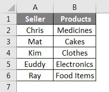
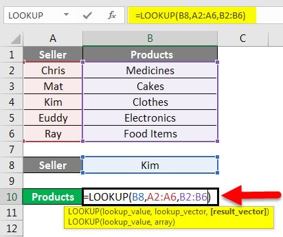
Consider the below table containing details of sellers and their products. You want to find out the product sold by Kim.
Solution:
Step 1: Click on Cell B10
Step 2: Enter the formula “=LOOKUP(B8,A2:A6,B2:B6)” as shown below.
Step 3: Press “Enter”
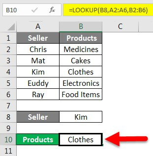
The result, “Clothes,” is displaced. Thus, Kim sold Clothes.
Explanation of the formula: “=Lookup(B8,A2:A6,B2:B6)”
This LOOKUP function searches the lookup_value, Cell B8 (Kim), in the lookup_vector, A2:A6, and returns the value in the same row from the result_vector, B2:B6. In simple terms, the value of Cell B8 is present in A4, and the function returns the value from the same position in another column, B4. The final output is Clothes.
Example #2
Let’s take another example to understand the vector form of the LOOKUP function.
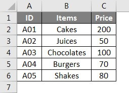
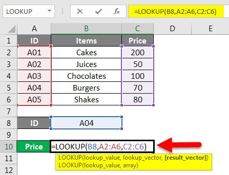
The below data consist of ID, Items, and their price, and you want to find out the price for ID A04. To search for a price, follow the steps of the solution.
Solution:
Step 1: Click on Cell B10
Step 2: Enter the formula “=LOOKUP(B8,A2:A6,C2:C6)” as shown below.
Step 3: Press “Enter” to get the result.
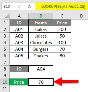
Output 70 is displayed as shown below. Hence, the price of ID A04 is 70.
Explanation of the formula: “=LOOKUP(B8,A2:A6,C2:C6)”
The lookup_value, A04, is first searched in the range of lookup_vector (A2 to A6). Here the lookup_value is A04; the lookup_vector is A2:A6, and the result_vector is C2:C6. The look_up value is in A5; now, the function returns the value in the same row from the result_vector range (B2:B6), i.e., B5. Thus, the output of the given formula is 70.
Example #3
How to search for a value in a one-row range?
In the above two examples, you have learned to use the vector form of the function to search for value in a single column. In this example, you will learn to search for deals in a one-row range.
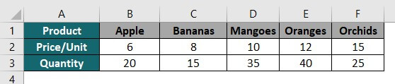
Consider the below table of products and their quantity arranged in a row. Now, you want to find the number of apples.
Solution:
Step 1: Click on Cell B7
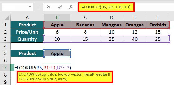
Step 2: Enter the formula “LOOKUP(B5, B1:F1, B3:F3)” as shown below.
Step 3: Press “Enter” to get the desired result.
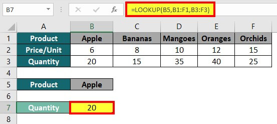
Output 20 is displaced in Cell B7. Thus, the quantity of apples is 20.
Example #4
How do you search value using the array form?
In all the above examples, we have used the vector form of the LOOKUP function. In this example, we will use the array form.
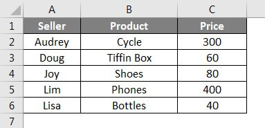
For instance, you have the below data and want to know the price of the product sold by Doug.
Solution:
Step 1: Click on Cell B9
Step 2: Enter the formula “=LOOKUP(B8,Al:C6)”, as shown below.
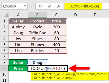
Step 3: Press “Enter” to see the result.
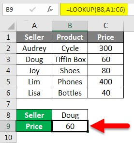
The result of the formula is 60. Thus, the price of the product sold by Doug is 60.
Explanation of the formula: “=LOOKUP(B8, A1:C6)”
Here, the lookup_value is B8, and the array range is A1: C6. The formula will search for the value of Cell B8 from Cell A1 to Cell C6 and returns the value corresponding to Cell B8.
Example #5
How to find a value in the last non-blank cell in a column?
In this example, you will learn to retrieve the last entry data, i.e., the last non-blank cell in a column, using the vector form of the LOOKUP function.
The syntax for retrieving the last value of a specific column is:
=Lookup(2,1/(column<>””), column)
Consider the below example. You need to find out the last entry in this table.

Solution:
Step 1: Click on Cell B8
Step 2: Enter the formula “=LOOKUP(2,1/(A2:A6<>””),A2:A6)” and press ”Enter”.

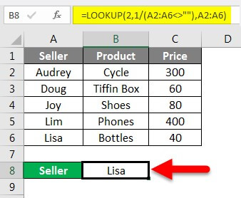
The output of the formula is Lisa. Thus, the last entry data in column A is Lisa.
Similarly, you can also find the last entry in the product and price columns. Enter the formula shown in the below image to get the desired result.
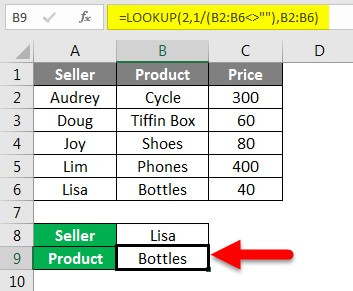
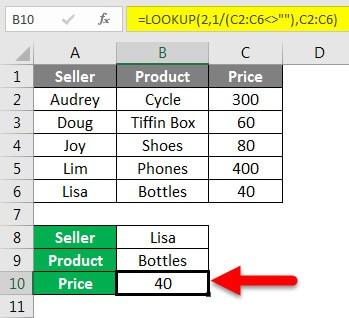
So, the last entry in the column product is Bottles, and the price is 40.
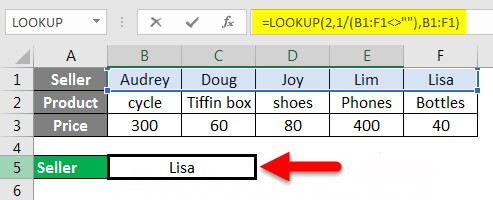
How to find a value in the last non-blank cell in a row?
In the previous example, you have learned to find the last entry in a specific column using the Lookup function. You will learn to see the previous entry in a particular row here.
The syntax for retrieving the last value of a specific row is:
“= Lookup(2,1/(Row<>””),Row)”
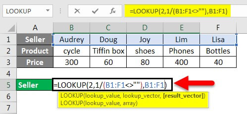
You have to find the last entry data in the Seller row in the data below.
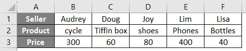
Solution: Enter the formula=” LOOKUP(2,1/(B1:F1<>”), B1:F1)” in the desired cell and press “Enter“.
Things to Remember
1. While Using the Vector Form of the LOOKUP Function
- The LOOKUP function with a result_vector provided will check for the lookup_value in the lookup_vector range and return the corresponding value from the result_vector.
- Without a result_vector, it will return the result value found from the lookup_vector.
- If the lookup_value cannot be found, the function returns the next smallest value or equal to the lookup_value.
- If the lookup_value is less than the lowest value in the lookup_vector, the function will display the #N/A error.
- The function will return the last value in the range of the lookup value that exceeds each vector value.
- If it cannot find the exact lookup_value, it searches for the next highest value that is lower than or equal to the lookup_value.
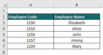
Let us learn about the above conditions through an example. The below data contains details of employee codes and their name.
|
Formula |
Description |
Result |
| =LOOKUP(1150,A3:A7,B3:B7) | The Lookup function finds the exact match of the lookup_value in column A. | Elizabeth |
| =LOOKUP(1156, A3:A7, B3:B7) | The function looks for the nearest value for 1156 and returns the value of 1157 | John |
| =LOOKUP(1151, A3:A7, B3:B7) | The function looks for the nearest value for 1151 and returns the value of 1150 | Elizabeth |
| =LOOKUP(1124,A3:A7,B3:B7) | lookup_value is smaller than all values present in A3:A7. | #N/A
|
| =LOOKUP(0, A3:A7, B3:B7) | The function looks for 0 and returns an error because 0 is less than the smallest value, 1150. | #N/A |
| =LOOKUP(1162, A3:A7, B3:B7) | The function looks up for value 1162 and returns the last value from column A. | Mary |
2. While Using the Array Form of the LOOKUP Function
- If the array range has multiple columns than rows (broader than taller), then the LOOKUP function will look for the lookup_value in the first row of the array (like HLOOKUP).
- If the array range has multiple rows than columns (taller than broader) or an equal number of rows and columns, then the LOOKUP function will look for the lookup_value in the first column (like VLOOKUP).
- In both cases, the LOOKUP function will return the very last value in the row or column of the array.
Essential Notes
- Sort the values in the lookup vector and result vector in ascending order, e., from A to Z if the values are in text and smallest to biggest if they are in numeric form.
- The LOOKUP function in Excel may provide incorrect results or errors if the data is unsorted.
- The LOOKUP function is not case-sensitive. It does not distinguish between text written in uppercase and lowercase.
- The lookup_vector and result_vector should be the same size when using the vector form of the LOOKUP function.
Frequently Asked Questions(FAQs)
Q1. What is the formula for lookup in Excel?
Answer: There are two types of lookup formulas in Excel.
- Vector form: The formula for the vector form of the lookup function is “=LOOKUP(lookup_value, lookup_vector, [result_vector]).”
- Array form: The formula for the array form of the lookup function is “=LOOKUP(lookup_value, array).”
Q2. Why do we use lookup in Excel?
Answer: Excel’s lookup function is useful for finding a specific record, closest match, or corresponding value to a given value.
Recommended Articles
This article is a tutorial for the LOOKUP Function in Excel. We have covered how to use the LOOKUP function for different conditions in Excel, practical examples, and a downloadable Excel template. You might also read our other recommended articles:
