Updated May 12, 2023
Excel TRANSPOSE Formula (Table of Contents)
TRANSPOSE Formula in Excel
Sometimes the data is not available in the manner we want. For example, it may be due to the system generating a report, or some people like to see the information differently than you prefer. One example is when the information is available horizontally, but you want to see the information vertically or vice-versa.
Microsoft Excel has an inbuilt function to tackle this issue known as “Transpose.” Transpose helps us to re-arrange the information in the manner we want. For example, it helps us to swap or switch columns to rows without re-typing the information. There are different ways to use the Transpose Formula in Excel. Either you can use this with the Copy-Paste function, or you can use the Transpose Formula.
How to Use TRANSPOSE Formula in Excel?
TRANSPOSE Formula in Excel is very simple and easy to use. Let’s understand how to use the TRANSPOSE Formula in Excel with the help of some examples.
Let’s look at the below example where I want to switch the information from Horizontal to Vertical.
Example #1
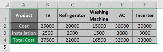
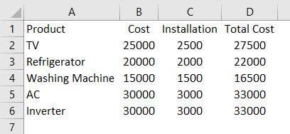
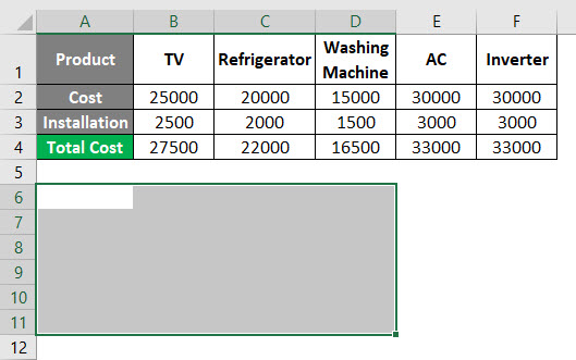
In this spreadsheet, I have given the cost and installation charges of some Electric appliances. The information is available in a Horizontal Manner. So I have to change the report orientation from Horizontal to vertical.

Now, to switch or swap the information from Horizontal to Vertical, we must follow the steps below.
Related Courses
Excel Training (21 Courses, 9+ Projects)
- Select the range of information that you need to swap or switch. In this example, A1:F4.
- Copy the Table (CTRL+C) and go to another sheet (or anywhere in the Excel sheet where you want the information) and Paste special values (CTRL+ALT+V).
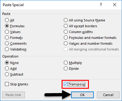
- After the special paste values, you will see the below options.
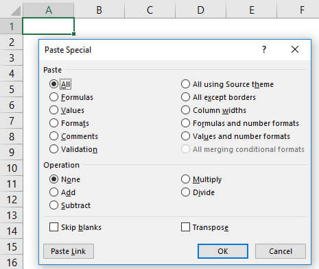
- As you can see, there are multiple options for Paste & Operation. In the paste area, there are two important options (Values and Formulas). Select Values if you just want to copy the values of data, and select Formulas if you want to copy the data with Formulas. Also, there is an additional option for Skip Blanks and Transpose.
- In this case, I am selecting Formulas because I need the data with formulas. So click on the Formula button.
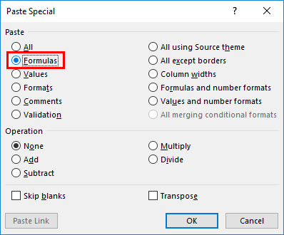
- In addition to the formula button, click on the Transpose button. So that it can paste the data with formulas, swap the information from Horizontal to vertical, and then click OK.
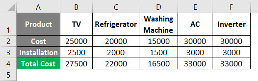
- Now you will see the information pasted vertically.
Introduction to Transpose Function
Now we have seen how to swap orientation with the help of the copy-paste feature, but there is a risk of creating duplicated data. So to avoid that, we can use the TRANSPOSE function in Excel. You will need to be a little careful while using the function.
The Transpose function must be entered as an array formula in a range with the same number of rows and columns as in the source data.
The values will also change in the Transpose Formula whenever the source information changes. This is the main difference between using the Transpose function and the Transpose with copy-paste feature. In the copy-paste feature, the values will not change if the source information changes. So Transpose function is more useful than the copy-paste feature.
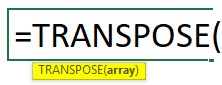
The syntax for the transpose Formula is:
Example #2
We will see the same example above and try to use the TRANSPOSE formula in Excel.
Please follow the below steps to use this function.
- You must first select some blank cells in the other direction as the original set of cells and select the same number of cells. In our example, we must select 24 cells in the opposite direction. As you can see in the below screenshot, I have selected 24 blank cells in the Vertical direction.
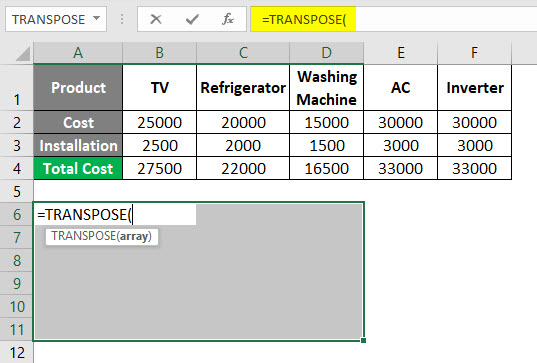
- Now be careful with this step because you need to insert the TRANSPOSE Formula in Cell A6 while all the blank cells are still selected. Please refer to the below screenshot on how to do this.
- The next step is to select the range of the original cells for which you need to change the orientation. In our example, the range is A1:F4. After selecting the range, don’t press ENTER because ENTER will not work with this function.
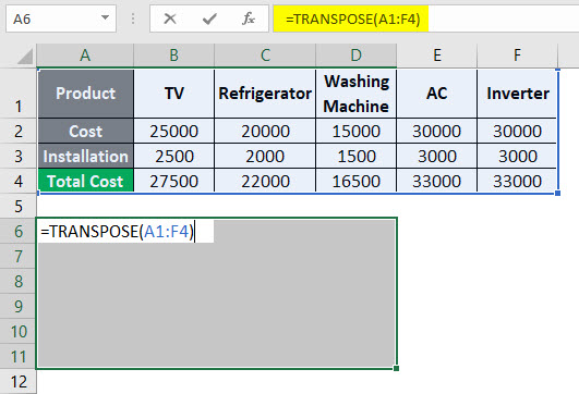
- So the last step in this function is to press CTRL + SHIFT + ENTER. The reason for doing this is because TRANSPOSE is an array function, and this is how an array function ends and not by pressing ENTER. An array is a function that can perform multiple calculations on one or more items in a cell.
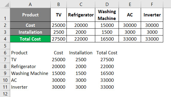
- After hitting the CTRL+SHIFT+ENTER, you will see the result below.
TRANSPOSE function with IF Condition
The transpose function can be used with other functions to get the desired results. So let’s try to use this with the IF Condition formula.
Example #3
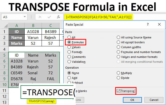
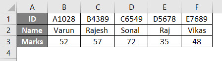
Suppose you have a report card of a few students available in the Horizontal orientation. For students who score below 50 or are absent, you want to transpose the information to be marked as Fail.
So we can use transpose Formula with IF condition like below.
=TRANSPOSE(IF(A1:F3<50,”FAIL”,A1:F3))
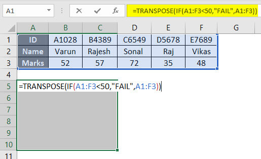
But make sure not to press ENTER and press CTRL+SHIFT+ENTER.
So after hitting the CTRL+SHIFT+ENTER, you can see the result below.
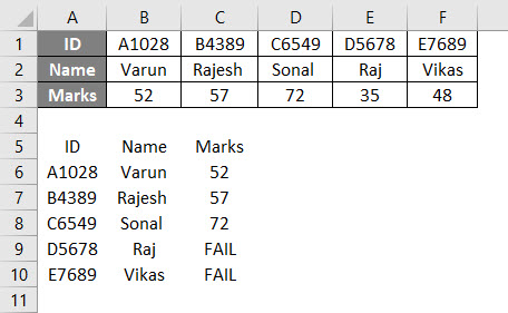
As you can see, Raj and Vikas scored less than 50, so they are marked as FAIL.
Things to Remember
- Make sure you select the same number of blank cells as the number of cells in source information while using the Transpose Formula.
- Ensure you do not press ENTER after inserting the Transpose Formula because the Transpose function is an Array function. Instead, it would be best if you pressed CTRL+SHIFT+ENTER.
- You can use the copy and paste feature for Transpose, which creates duplicate data. So when the values in source information change, the values are not updated.
Recommended Articles
This is a guide to the TRANSPOSE Formula in Excel. Here we have discussed calculating TRANSPOSE Formula in Excel, practical examples, and a downloadable Excel template. You may also look at the following articles to learn more –
