Updated May 8, 2023
SUMPRODUCT Formula in Excel
SUMPRODUCT formula in Excel is a function that simultaneously does multiplication and sum of cells. This formula multiplies the cell range/arrays and returns the sum of products in Excel.
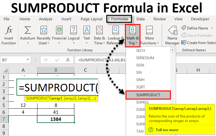
This function can be used as a workbook function. SUMPRODUCT can be found under Math and Trigonometry formulas in Excel. This function is present in all versions of Excel. This function is very commonly used in Excel. It can also be used in multiple ways, which are described in the below examples as well. This function is helpful in financial analysis as well. It compares data in several arrays and also calculates data with different criteria.
Below is the formula or Syntax of SUMPRODUCT in Excel :
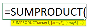
In the above syntax, array1 and array2 are the cell ranges or an array whose cells we want to multiply and add. If we only have one array, the function will only sum the cell range or array. So for the function to give the sum of products, we should have 2 arrays. While in previous versions of Excel, we had 30 arrays. We can have a maximum of 255 arrays in a newer version of Excel.
Suppose we have two arrays and want to know the sum of their products.
=SUMPRODUCT({2,4,5,6},{3,7,8,9})
= (2*3)+(4*7)+(5*8)+(6*9)
= 6+28+40+54
= 128
This is how first the elements of the 1st array are multiplied with the first element of a 2nd array and so on. And then their product is added.
How to Use SUMPRODUCT Formula in Excel?
SUMPRODUCT Formula in Excel is very simple and easy to use. Let us now see how to use the SUMPRODUCT Formula in Excel with the help of some examples. These examples will surely help you with a clear understanding of the function.
Excel SUMPRODUCT Formula – Example #1
In our first example, we will calculate the SUMPRODUCT of two cell ranges. Below is the sample data.
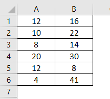
Now we will calculate the SUMPRODUCT of these arrays. We will write the formula below:
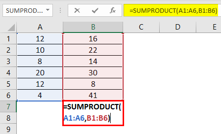
Press Enter to see the result.
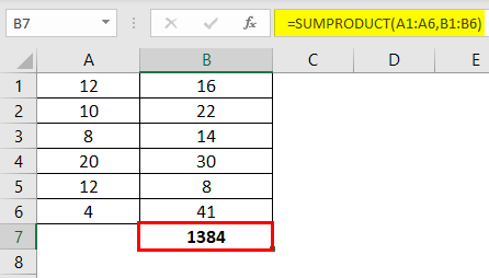
Here is the explanation of the above formula:
=(12*16)+(10*22)+(8*14)+(20*30)+(12*8)+(4*41)
= 192+220+112+600+96+164
=1384
Excel SUMPRODUCT Formula – Example #2
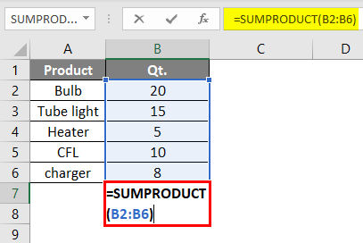
Here we have data for Electrical products. We will now calculate their SUMPRODUCT.
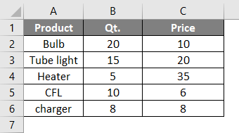
Now, we will write the formula:
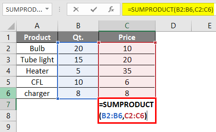
Press Enter to see the result.
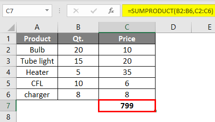
In the above formula, the first cell of the first array (Qt.) is multiplied by the second array’s first cell (Price). The second cell of the first array will be multiplied by the second cell of the second array, and so on, until the arrays’ fifth cell. After the arrays are multiplied, their product is added up to give the SUMPRODUCT, which is 799.
In case we have only one array, as shown below and we write the formula:
Press Enter to see the result.
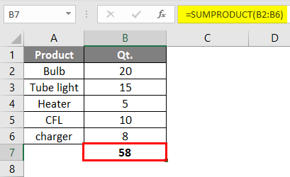
The function will now give the result of a SUM function. That is the sum of all cells in the range.
Excel SUMPRODUCT Formula – Example #3
In this example, we will see how the function works with single or multiple criteria.
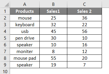
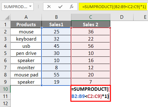
Suppose we have products in column A, sales 1 for the 1st quarter and sales 2 for the 2nd quarter, and we wish to find out the number of products sold less in sales 1 compared to sales 2.
Below is the sample sales data.
We will now write the formula below:
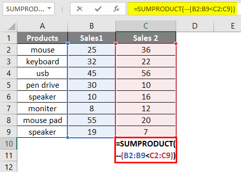
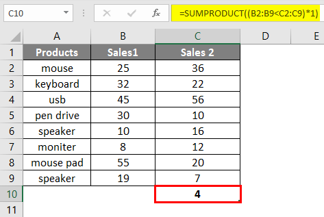
Press Enter, and we will see the below result.

Here 4 products in sales 1 are sold less compared to sales 2. The double-negative (–) in the formula is used to convert True and False into 1 and 0 in Excel.
Also, there is another way of doing this.
Press Enter, and you will get the same result 4.
Excel SUMPRODUCT Formula – Example #4
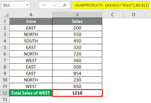
Here we have another example in which we have sales data per zone, and we want to know the sales for a particular zone, say West zone.
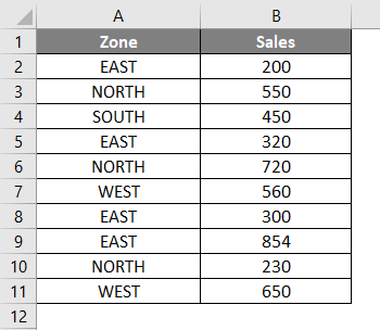
Now we will write the formula in cell B12.
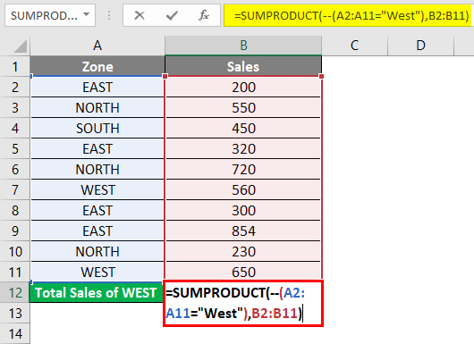
Press Enter to see the result.
As mentioned above, we use a double negative mark to convert logical values (True and false) into numeric values (0, 1). We can do the same with a “*” sign.
We can also write the formula as shown below using “*” instead of “- -”
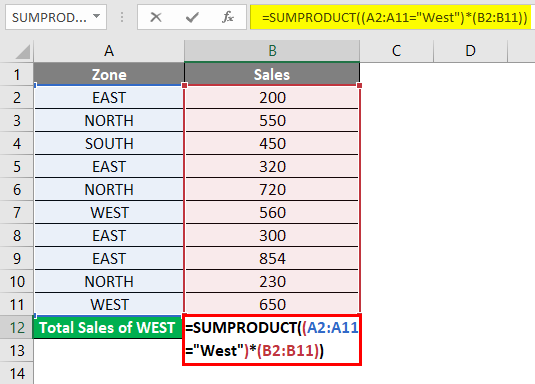
Press Enter to see the result.

Excel SUMPRODUCT Formula – Example #5
We will now look into using the SUMPRODUCT function in multiple criteria.
Let’s say we have region-wise sales data of bikes.
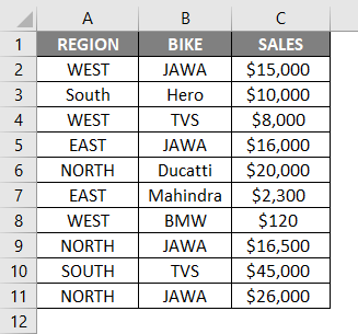
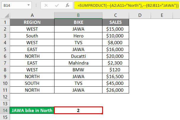
Suppose we want to count the sales of JAWA bikes in the North region. We can do so by writing the Excel SUMPRODUCT formula below:
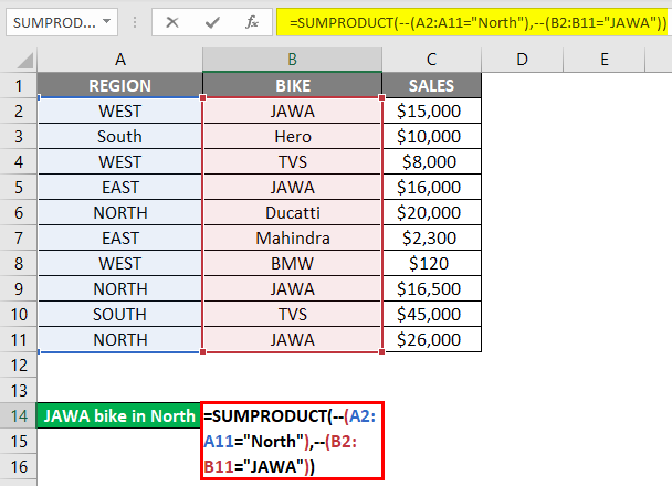
Press Enter to know the count of JAWA bikes sold in North.
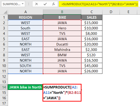
Another way of writing the above formula is shown below:
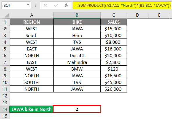
It will also give the same result. Here we have used the * sign instead of the – sign to convert True and False into 0 and 1.
Press Enter to see the result.
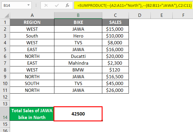
Taking the above scenario, we now want to know the total sales of JAWA bikes in the North region.
For this, we will write the SUMPRODUCT formula in Excel as below:
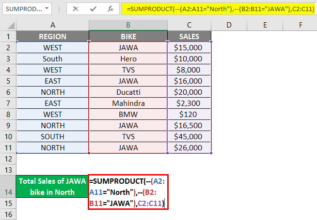
Press Enter to know the total sales.
Also, we can write the above formula as below:
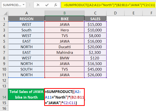
Press Enter to see the results.
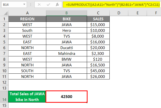
An asterisk (*) sign is an OR operator in the above example.
Excel SUMPRODUCT Formula – Example #6
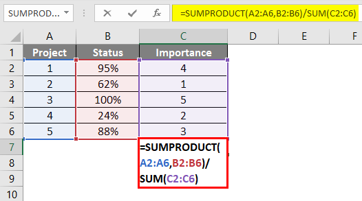
A SUMPDOUCT formula is also used to calculate the weighted average in Excel. The formula to calculate the weighted average is =SUMPRODUCT(value, weight)/SUM(weights)
Let’s understand this better with this example:
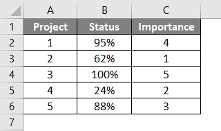
Here we have 5 different projects, their completion status, and their importance (rankings). We will now write the formula for a weighted average using the SUMPRODUCT function.
Press Enter to see the result.
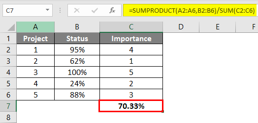
Here is how we calculate the weighted average.
Going through all the above examples will give you a better understanding of the function and its implications in different scenarios.
Things to Remember
- The array of arguments should have the same size. If they are not the same size or dimensions, you will get #VALUE! Error.
- The arrays should not contain text or non-numeric values. Because then all such cells will be treated as 0’s.
- In prior versions of Excel, you could only provide up to 30 arrays as arguments.
- If you have one array or have not provided the second array, the function will return the sum of that single array.
- If the arguments in the function are logical (True and False), they must be converted into numeric values (0, 1). This can be done by adding — sign as shown in the above examples.
- This function does not support wildcard characters like “*” and “?”.
- SUMPRODUCT Formula can even give results from a closed workbook in Excel.
Recommended Articles
This has been a guide to SUMPRODUCT Formula in Excel. Here we discuss how to use SUMPRODUCT Formula in Excel along with Excel examples and a downloadable Excel template. You can also go through our other suggested articles –
