Introduction to Linear Model in R
A statistical or mathematical model that is used to formulate a relationship between a dependent variable and single or multiple independent variables called as, linear model in R. The criteria is that the variables involved in the formation of model meet certain assumptions as necessary prerequisites prior model building and that the model has certain important elements as its parts, which are formula, data, subset, weights, method, model, offset etc. It is not necessary that all have to be used every time, but only those that are sufficient and essential in the given context.
Advantages of Linear Model:
- Helps us to understand the type and nature of the data.
- Helps us to predict the data.
- Helps us to make statistical inferences from data.
Now we will learn about linear regression basically it is a statistical method used to create these models. The main objective of this model is to explain the relationship between the dependent variable and the independent variable.
Syntax of Linear Model in R
Here is the syntax of the linear model in R which is given below.
Syntax:
lm(formula, data, subset, weights, na.action,

method = "qr", model = TRUE, x = FALSE, y = FALSE, qr = TRUE,

singular.ok = TRUE,offset, ...)
Here are the parameters of the linear model which are explained below:
- Formula: Here we have to enter the variables of our dataset, basically, those variables where we are planning to trace out whether any relationship exists between them or not. The format should be fixed like (Dependent variable ~ Independent variables). Eg (Distance ~ Speed), (Demand~Price), etc.
- Data: It is used when we have to pass an optional list of data, data frame or environment.
- Subset: It helps us to define the data when we have to use a subset of the observations.
- Weights: It accepts only numeric vector or “NULL” command. If it is not null, “WLS (Weighted least squares)” is used with weights or if Null then OLS (ordinary least squares) is used.
- Na.action: It will give the instruction of what should be done when the data points have NA values, like na.fail, na.omit, na.exclude, etc.
- Method: It is used for fitting.
- Model: It is a logical vector if it is TRUE the corresponding components of the fit are returned.
- X: It is a logical vector if it is TRUE the corresponding components of the fit are returned.
- Y: It is a logical vector if it is TRUE the corresponding components of the fit are returned.
- qr: It is a logical vector if it is TRUE the corresponding components of the fit are returned.
- ok: It is also a logical vector if it is FALSE then singular fits are the error.
- Offset: It can be NULL, numerical vector or matrix. This is used to specify an a priori known component to be included in the linear predictor during fitting.
Types of Linear Model in R
Let’s now discuss different types of linear models which are as follows:
1. Simple Linear Regression
This model helps us to explain a relationship between one dependent variable and one independent variable. With the help of it, we can also predict the data, by providing the input values. In general, the dependent variable is also known as the response variable, regressand, observed variable, responding variable, measured variable, explained variable, experimental variable, outcome variable, and/or output variable). And independent variable known as a controlled variable, regressors, explanatory variable, manipulated variable, exposure variable, and/or input variable. The equation for the simple linear regression model is:
Where β1 is an intercept, β2 is a slope and ϵ is an error term. We will use the “USArrest” data set.
| Murder arrests (per 100,000) | Assault arrests (per 100,000) | Percent urban population | Rape arrests (per 100,000) | |
| Alabama | 13.2 | 236 | 58 | 21.2 |
| Alaska | 10 | 263 | 48 | 44.5 |
| Arizona | 8.1 | 294 | 80 | 31 |
| Arkansas | 8.8 | 190 | 50 | 19.5 |
| California | 9 | 276 | 91 | 40.6 |
| Colorado | 7.9 | 204 | 78 | 38.7 |
| Connecticut | 3.3 | 110 | 77 | 11.1 |
| Delaware | 5.9 | 238 | 72 | 15.8 |
| Florida | 15.4 | 335 | 80 | 31.9 |
| Georgia | 17.4 | 211 | 60 | 25.8 |
| Hawaii | 5.3 | 46 | 83 | 20.2 |
| Idaho | 2.6 | 120 | 54 | 14.2 |
| Illinois | 10.4 | 249 | 83 | 24 |
| Indiana | 7.2 | 113 | 65 | 21 |
| Iowa | 2.2 | 56 | 57 | 11.3 |
| Kansas | 6 | 115 | 66 | 18 |
| Kentucky | 9.7 | 109 | 52 | 16.3 |
| Louisiana | 15.4 | 249 | 66 | 22.2 |
| Maine | 2.1 | 83 | 51 | 7.8 |
| Maryland | 11.3 | 300 | 67 | 27.8 |
| Massachusetts | 4.4 | 149 | 85 | 16.3 |
| Michigan | 12.1 | 255 | 74 | 35.1 |
| Minnesota | 2.7 | 72 | 66 | 14.9 |
| Mississippi | 16.1 | 259 | 44 | 17.1 |
| Missouri | 9 | 178 | 70 | 28.2 |
| Montana | 6 | 109 | 53 | 16.4 |
| Nebraska | 4.3 | 102 | 62 | 16.5 |
| Nevada | 12.2 | 252 | 81 | 46 |
| New Hampshire | 2.1 | 57 | 56 | 9.5 |
| New Jersey | 7.4 | 159 | 89 | 18.8 |
| New Mexico | 11.4 | 285 | 70 | 32.1 |
| New York | 11.1 | 254 | 86 | 26.1 |
| North Carolina | 13 | 337 | 45 | 16.1 |
| North Dakota | 0.8 | 45 | 44 | 7.3 |
| Ohio | 7.3 | 120 | 75 | 21.4 |
| Oklahoma | 6.6 | 151 | 68 | 20 |
| Oregon | 4.9 | 159 | 67 | 29.3 |
| Pennsylvania | 6.3 | 106 | 72 | 14.9 |
| Rhode Island | 3.4 | 174 | 87 | 8.3 |
| South Carolina | 14.4 | 279 | 48 | 22.5 |
| South Dakota | 3.8 | 86 | 45 | 12.8 |
| Tennessee | 13.2 | 188 | 59 | 26.9 |
| Texas | 12.7 | 201 | 80 | 25.5 |
| Utah | 3.2 | 120 | 80 | 22.9 |
| Vermont | 2.2 | 48 | 32 | 11.2 |
| Virginia | 8.5 | 156 | 63 | 20.7 |
| Washington | 4 | 145 | 73 | 26.2 |
| West Virginia | 5.7 | 81 | 39 | 9.3 |
| Wisconsin | 2.6 | 53 | 66 | 10.8 |
| Wyoming | 6.8 | 161 | 60 | 15.6 |
Now we will find the relationship between the Assault variable and the Urban population.
>dataset = USArrests
>Linear_relationship1 = lm(Assault~ UrbanPop, data=dataset)
> Linear_relationship
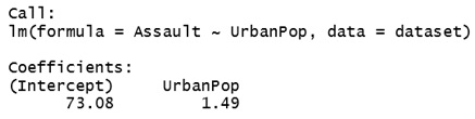
Equation looks like:
Now we have intercept and slope also, Assault = 73.08 + 1.49(UrbanPop). Here we have a linear model equation, we have to supply the inputs in the form of “UrbanPop”, and the model equation will automatically predict the value of “Assualt” for us. Let’s take another example of this model, now we will run this model on Murder variable and Urban Population variable.
>View(USArrests)
>Linear_relationship2= lm(Murder~ UrbanPop, data=dataset)
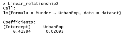
Equation looks like:
Now we have intercept and slope also, Murder= 6.41594 + 0.02093(UrbanPop). Here we have a linear model equation, we have to supply the inputs in the form of “UrbanPop”, and the model equation will automatically predict the value of “Murder” for us.
2. Multiple Linear Regression
In this model, we will have one dependent variable and multiple independent variables. Multiple independent variables are used in this model to predict one dependent variable. Let’s take an example of this model. Here also we will use the “USArrests” dataset.
Dependent variable = Urban Population
Independent variable = Assault, Rape, and Murder
>Multiple_Linear_Relationship = lm(UrbanPop~ Assault+Rape+Murder , data=dataset)
>Multiple_Linear_Relationship
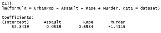
The equation looks like:
Now we have intercept and slope also, UrbanPop= 52.8419 + 0.0519(Assault) + 0.6984(Rape) – 1.4115(Murder)
Conclusion
The linear model generally works around two parameters: one is slope which is often known as the rate of change and the other one is intercept which is basically an initial value. These models are very common in use when we are dealing with numeric data. Outcomes of these models can easily break down to reach over final results. Therefore, researchers, academicians, economists prefer these models.
Recommended Articles
This is a guide to Linear Model in R. Here we discuss the types, syntax, and parameters of the Linear Model in R along with its advantages. You can also go through our other suggested articles to learn more –
