Updated July 5, 2023
Definition of Arima Model
Arima, in short term as Auto-Regressive Integrated Moving Average, is a group of models used in R programming language to describe a given time series based on the previously predicted values and focus on the future values. The Time series analysis is used to find the behavior of data over a time period. This model is the most widely used approach to forecast the time series.Arima() function is used to process the model.
Syntax:
Auto.arima()
This searches for order parameters.
How Arima model works in R?
ARIMA being an easier model in predicting a future value in series, takes time series data which are equally spaced points in a time(a pattern of value, rate of change of growth, outliers, or noise between the time points). Maximum Likehood Estimation (MLE) is used to estimate the ARIMA model. The model takes up three important parameters: p,d,q, respectively.MLE helps to maximize the likehood for these parameters when calculating parameter estimates.
ARIMA(p,d,q)
p- is the order of Auto-regressive or linear model
q – is the order of Moving Average/ number of lagged values
d- difference value to make the time series stationary from non-stationary. So we perform ARMA here, not ARIMA(means no Integration). The improvement over ARIMA is Seasonal ARIMA.
Now let us see how these three parameters bound each other and, lastly, the plots of ACF and PACF. As AR uses its lag errors as predictors. And works best when the used predictor is not independent of each other. The Model works on two important key concepts:
1. The Data series as input should be stationary.
2. As ARIMA takes past values to predict the future output, the input data must be invariant.
Implementation Steps:
1. Load the data set after installing the package forecast.
2. The Steps of Pre-processing are done, which creates a separate time-series or timestamp.
3. Making Time-series stationary and check the required transformations.
4. The difference value ‘d’ will be performed.
5. The core important step in ARIMA is plotting ACF and PACF.
6. Determine the two parameters p and q from the plots.
7. The previously created value fits the Aroma model and predicts the future values. The Fitting Process is also named as Box-Jenkins Method.
8. Doing Validation.
auto. Arima() function is used for automatic prediction and ARIMA Models. This function uses unit root tests, minimization of the AIC and MLE to obtain an ARIMA model. To make the series stationary, we need to differentiate a previous value from the current value.
d= pval-cval, if the value is already stationary the d=0.
predict() – Used to predict the model based on the results of the various fitting model used.
In this section, we will use graphs and plots using data sets to forecast the time series through ARIMA. The following sections analyse the forecast for the next coming years.
Working Process
Following Steps to be taken in exploring the model:
a. Exploratory Analysis
b. Fit
c. Diagnostic Measures
The best model selection process is necessary as in industrial cases, a lot of time series need to be forecasted.
1. Doing Time Series Data Modelling in R that converts the raw data into a time series format using the following command. If the dataset is already in time series ts() is not needed.
ts(data[,2],start = c(start time,1),frequency = numeric value)
// ts gives the daily, weekly, monthly observation of data. Start Gives start time to evaluate maybe a year. If it is a monthly schedule, the frequency value would be 12.
Examples
All the given R codes are executed in RStudio To plot values for future predictions.
Example #1: With Sale on the Textile dataset
Here is the step-by Step Process to Forecast the scenario through ARIMA Modeling. The Case Study I have used here is a textile sale data set. I have attached the file separately.
Code:
Step-1: Loading necessary R packages and Data set for implementation
data=read.csv('C:/sale.csv')

data = ts(data[,2],start = c(2005,1),frequency = 12)

plot(data, xlab='Year on sale', ylab = 'Number of Textile sold')
Step-2:
plot(diff(data),ylab='Differenced Textile Sold')
And the Plot Would be:
Step-3: Carrying Log Transform Data
plot(log10(data),ylab='Log (Number of Textile sold)')
Now the series looks like
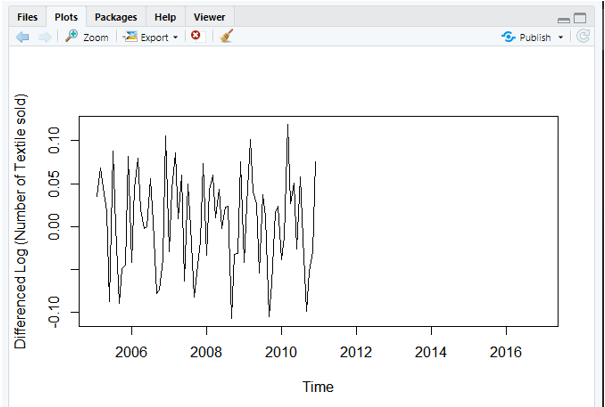
Step-4: Difference value
plot(diff(log10(data)),ylab='Differenced Log (Number of Textile sold)')
Step-5: Evaluate and iterate
require(forecast)

> ARIMAfit = auto.arima(log10(data), approximation=FALSE,trace=FALSE)

> summary(ARIMAfit)

Series: log10(data)

ARIMA(0,1,1)(1,1,0)[12]
Coefficients:

ma1 sar1

-0.5618 -0.6057

s.e. 0.1177 0.1078

sigma^2 estimated as 0.000444: log likelihood=142.17

AIC=-278.34 AICc=-277.91 BIC=-272.11

Training set error measures:

ME RMSE MAE MPE

Training set 0.000213508 0.01874871 0.01382765 0.009178474

MAPE MASE ACF1

Training set 0.5716986 0.2422678 0.0325363
Step-6 : To examine P and Q values we need to execute acf() and pacf() which is an autocorrelation function.
Example 2
library(forecast)
png(file = "TimeSeries1.png")
plot(CO2, main = "Plot with no forecasting",
col.main = "yellow")
dev.off()
png
2
png(file = "TimeSeries2.png")
fit <- auto.arima(co2)
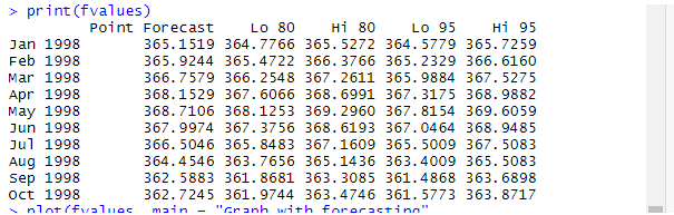
fvalues <- forecast(fit, 10)
print(fvalues)
plot(fvalues, main = " Plot with forecasting",",
col.main = "red")
dev.off()
png
2
Explanation
By executing the above code in Rstudio, we get the following outputs. Here the next 10 values are predicted in Co2 datasets using forecast ().
Output:
Example #3: Using a car-sale dataset
library(forecast)
library(Metrics)
Attaching package: ‘Metrics’
The following object is masked from ‘package:forecast’:
accuracy
Warning message:
package ‘Metrics’ was built under R version 3.6.3
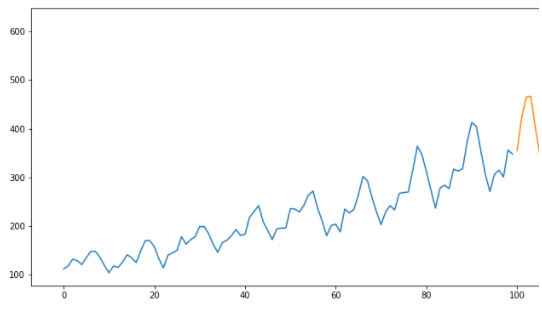
data = read.csv('https://raw.githubusercontent.com/jbrownlee/Datasets/master/monthly-car-sales.csv')
valid = data[51:nrow(data),]
train = data[1:50,]
valid = data[51:nrow(data),]
train$Month = NULL
model = auto.arima(train)
summary(model)
Series: train
ARIMA(2,0,2) with non-zero mean
Coefficients:
ar1 ar2 ma1 ma2 mean
0.9409 -0.6368 -0.0249 0.4868 11921.2100
s.e. 0.1837 0.1611 0.2254 0.1606 636.7033
sigma^2 estimated as 5124639: log likelihood=-455.41
AIC=922.82 AICc=924.78 BIC=934.3
Training set error measures:
ME RMSE MAE MPE MAPE MASE
Training set 21.53119 2147.598 1627.823 -3.37804 15.03798 0.6857703
ACF1
Training set 0.02558285
forecast = predict(model,40)
rmse(valid$monthly-car-sales, forecast$pred)
Output:
Conclusion
Coming to an end, the ARIMA model helps in predicting future values in Time Series, which helps to optimize business decisions. So we have covered a lot of basic introduction on forecasting and AR, MR models. Time series forecasting is the primary skill, and data scientists would expect to forecast the values of month-on-month expenditures.
Recommended Articles
This is a guide to Arima Model in R. Here, we discuss the Definition, syntax, How the Arima model works in R? for example, with code implementation. You may also have a look at the following articles to learn more –
