
Introduction to Multiple Linear Regression in R
Multiple Linear Regression is one of the data mining techniques to discover the hidden pattern and relations between the variables in large datasets. Multiple Linear Regression is one of the regression methods and falls under predictive mining techniques. It is used to discover the relationship and assumes the linearity between target and predictors. However, the relationship between them is not always linear. Hence, it is important to determine a statistical method that fits the data and can be used to discover unbiased results. Multiple linear regression is an extended version of linear regression and allows the user to determine the relationship between two or more variables, unlike linear regression where it can be used to determine between only two variables. In this topic, we are going to learn about Multiple Linear Regression in R.
Syntax
Lm() function is a basic function used in the syntax of multiple regression. This function is used to establish the relationship between predictor and response variables.
lm( y ~ x1+x2+x3…, data)
The formula represents the relationship between response and predictor variables and data represents the vector on which the formulae are being applied.
For models with two or more predictors and the single response variable, we reserve the term multiple regression. There are also models of regression, with two or more variables of response. Such models are commonly referred to as multivariate regression models. Now let’s look at the real-time examples where multiple regression model fits.
For example, a house’s selling price will depend on the location’s desirability, the number of bedrooms, the number of bathrooms, year of construction, and a number of other factors. A child’s height can rely on the mother’s height, father’s height, diet, and environmental factors.
Now let’s see the general mathematical equation for multiple linear regression
Y= a + b1x1 + b2x2 +…bnxn
- Where Y represents the response variable
- a, b1, b2, and bn are coefficients
- and x1, x2, and xn are predictor variables.
Examples of Multiple Linear Regression in R
The lm() method can be used when constructing a prototype with more than two predictors. Essentially, one can just keep adding another variable to the formula statement until they’re all accounted for. In this section, we will be using a freeny database available within R studio to understand the relationship between a predictor model with more than two variables. This model seeks to predict the market potential with the help of the rate index and income level.
Example #1 – Collecting and capturing the data in R
For this example, we have used inbuilt data in R. In real-world scenarios one might need to import the data from the CSV file. Which can be easily done using read.csv.
Syntax: read.csv(“path where CSV file real-world\\File name.csv”)
Example #2 – Check for Linearity
Before the linear regression model can be applied, one must verify multiple factors and make sure assumptions are met. Most of all one must make sure linearity exists between the variables in the dataset. One of the fastest ways to check the linearity is by using scatter plots.
In our dataset market potential is the dependent variable whereas rate, income, and revenue are the independent variables. Now let’s see the code to establish the relationship between these variables.
# extracting data from freeny database

data("freeny")

# plotting the data to determine the linearity

plot(freeny, col="navy", main="Matrix Scatterplot")
Output:
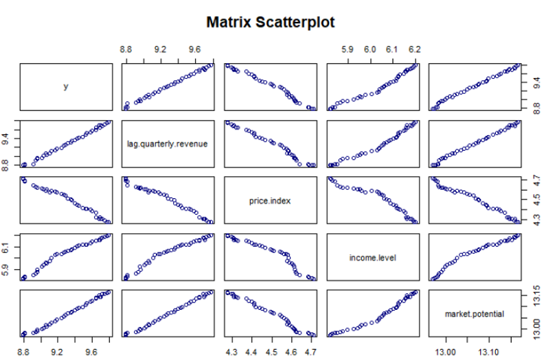
From the above scatter plot we can determine the variables in the database freeny are in linearity.
# Constructing a model that predicts the market potential using the help of revenue price.index

and income.level

> model <- lm(market.potential ~ price.index + income.level, data = freeny)

> model
Output:
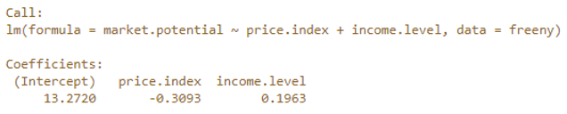
The sample code above shows how to build a linear model with two predictors. In this example Price.index and income.level are two
predictors used to predict the market potential. From the above output, we have determined that the intercept is 13.2720, the
coefficients for rate Index is -0.3093, and the coefficient for income level is 0.1963. Hence the complete regression Equation is market
potential = 13.270 + (-0.3093)* price.index + 0.1963*income level.
model <- lm(market.potential ~ price.index + income.level, data = freeny)
model
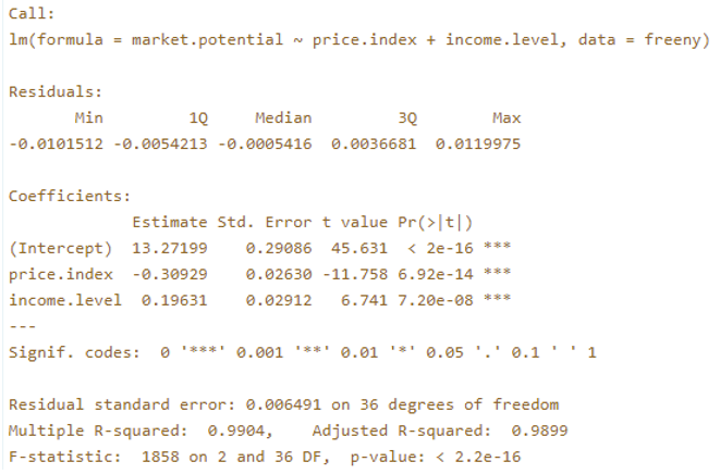
using summary(OBJECT) to display information about the linear model
summary(model)
Output:
Summary evaluation
1. Adjusted R squared
This value reflects how fit the model is. Higher the value better the fit. Adjusted R-squared value of our data set is 0.9899
2. P-value
Most of the analysis using R relies on using statistics called the p-value to determine whether we should reject the null hypothesis or
fail to reject it. With the assumption that the null hypothesis is valid, the p-value is characterized as the probability of obtaining a
result that is equal to or more extreme than what the data actually observed. P-value 0.9899 derived from out data is considered to be
statistically significant.
3. Std.Error
The standard error refers to the estimate of the standard deviation. The coefficient of standard error calculates just how accurately the
model determines the uncertain value of the coefficient. The coefficient Standard Error is always positive. One can use the coefficient
standard error to calculate the accuracy of the coefficient calculation.
The analyst should not approach the job while analyzing the data as a lawyer would. In other words, the researcher should not be
searching for significant effects and experiments but rather be like an independent investigator using lines of evidence to figure out
what is most likely to be true given the available data, graphical analysis, and statistical analysis.
Conclusion
In this article, we have seen how the multiple linear regression model can be used to predict the value of the dependent variable with the help of two or more independent variables. The initial linearity test has been considered in the example to satisfy the linearity. As the variables have linearity between them we have progressed further with multiple linear regression models. We were able to predict the market potential with the help of predictors variables which are rate and income.
Recommended Articles
This is a guide to Multiple Linear Regression in R. Here we discuss how to predict the value of the dependent variable by using multiple linear regression model. You may also look at the following articles to learn more –
