Updated August 24, 2023
Dynamic Chart in Excel
Dynamic Chart in Excel automatically updates when we insert a new value in the selected table. First, we need to create a dynamic range in Excel to create a dynamic chart. In the first step, we must change the data into Table format from the Insert menu tab. That created table will automatically switch to the format we need, and the chart using that table will be a Dynamic chart, and the chart created by using such type of data will update with the format we need.
We need to delete every previously used data if we want to keep fix set of data in Charts.
The two main methods used to prepare a dynamic chart are as follows:
- By Using Excel Table
- Using Named Range
How to Create a Dynamic Chart in Excel?
Dynamic Chart in Excel is very simple and easy to create. Let’s understand the working of Dynamic Chart in Excel with Some Examples.
Example #1 – By Using Excel Table
This is one of the easiest methods to make a dynamic chart in Excel, available in the Excel versions of 2007 and beyond. The basic steps to follow are:
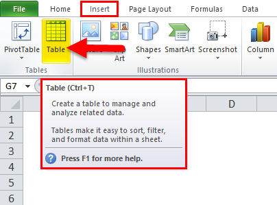
- Create a table in Excel by selecting the table option from the Insert
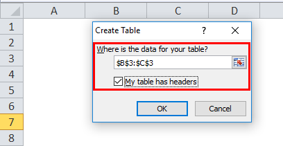
- A Dialog box will appear to give the Range for the Table, and Select the option ‘ My Table has Headers ‘
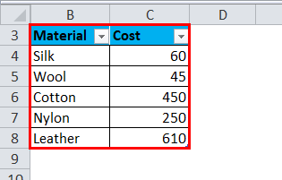
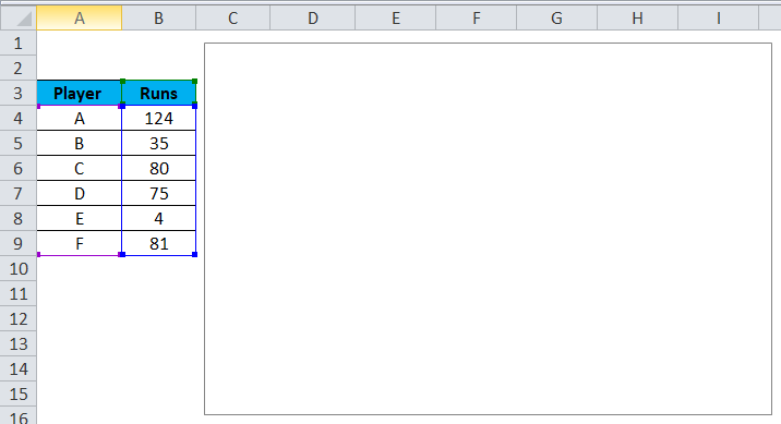
- Enter the data in the selected table.
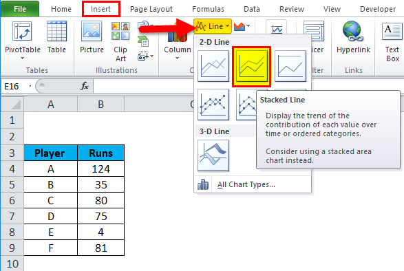
- Select the table and insert a suitable chart for it.
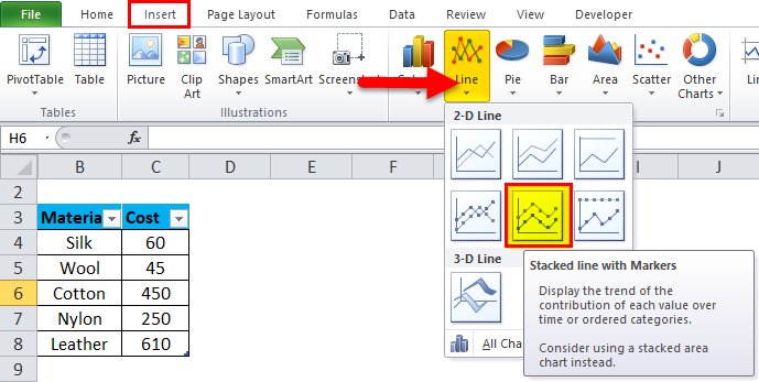
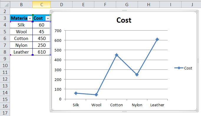
- A stacked Line with the Markers Chart is inserted. Your chart will look like this as given below:
- Change the data in the table, which will change the chart.
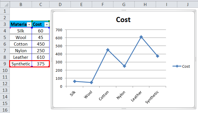
In step 4, it can observe that the graph is automatically updated after changing the dynamic input range of the column. There is no need to change the chart, which is an efficient way to analyze the data.
Example #2 – By Using Named Range
This method is used when the user uses an older version of Excel, such as Excel 2003. It is easy to use but not as flexible as the table method used in Excel for the dynamic chart. There are 2 steps in implementing this method:
- Creating a dynamic named range for the dynamic chart.
- Creating a chart by using named ranges.
Creating a Dynamic Named Range for the Dynamic Chart
In this step, an OFFSET function (Formula) is used to prepare a dynamic named range for the particular dynamic chart. This OFFSET function will return a cell or range of cells specified to the referred rows and columns. The basic steps to be followed are:
- Make a table of data as shown in the previous method.
- From the ‘Formulas’ tab, click on ‘Name Manager’.
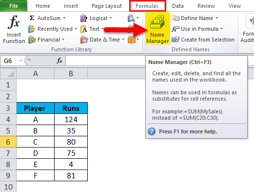
- A Name Manager Dialog box will appear in that Click on “New”.
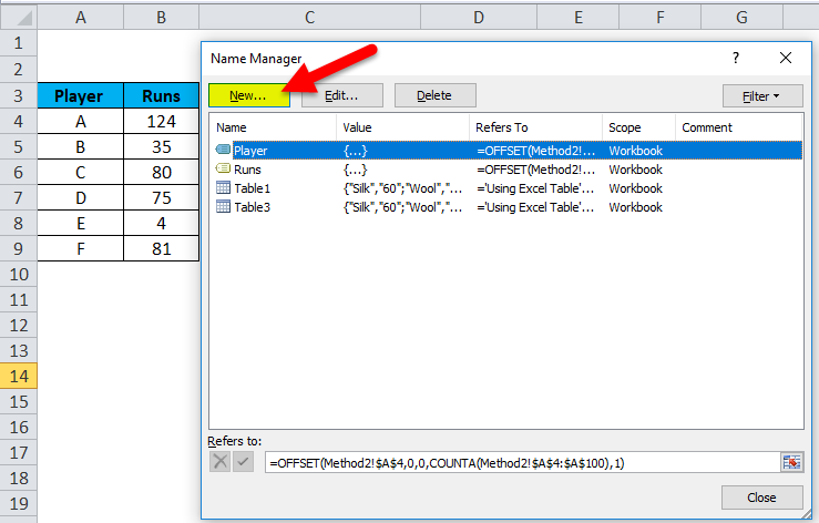
- In the appeared dialogue box from the ‘Name Manager’ option, assign the name in the tab for the name option, and enter the OFFSET formula in the ‘ Refers To ‘ tab.
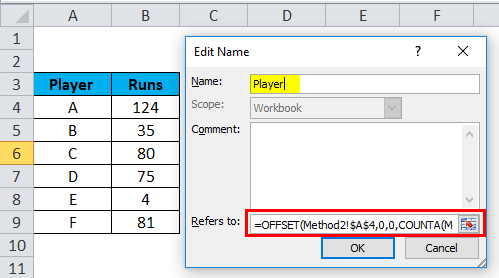
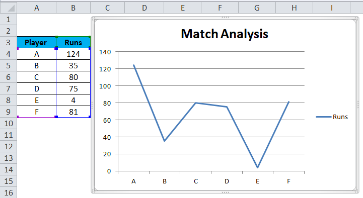
As two names have been taken in the example (Player and Runs), two name ranges will define, and the OFFSET formula for both names will be as follows:
- Player =OFFSET($A$4,0,0,COUNTA($A$4:$A$100),1)
- Runs =OFFSET($B$4,0,0,COUNTA($B$4:$B$100),1)
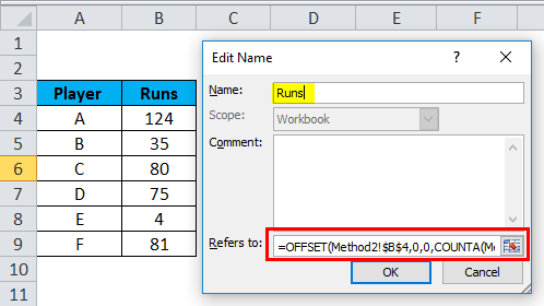
The formula used here makes use of the COUNTA function as well. It gets the count of some non-blank cells in the target column, and the counts go to the height argument of the OFFSET function, which instructs the number of rows to return. In Step 1 of method 2, defining a named range for the dynamic chart is demonstrated, where a table is made for two names, and the OFFSET formula is used to define the range and create name ranges to make the chart dynamic.
Creating a Chart by Using Named Ranges
In this step, a chart is set and inserted, and the created name ranges represent the data and make the chart dynamic. The steps to be followed are:
- Select the ‘Line’ chart option from the Insert tab.
- A Stacked Line chart is inserted.
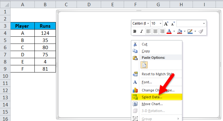
- Select the entire chart, either right-click or go to the ‘select data’ option, or from the ‘Design’ tab, go to the ‘select data’ option.
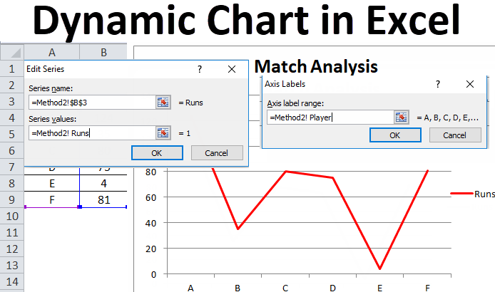
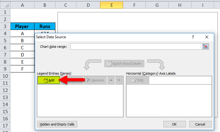
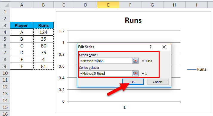
- After selecting the data option, the ‘Select Data Source dialogue box will appear. In that, click on the ‘Add’ button.
- From the Add option, another dialogue box will appear. In that, in the series name tab, select the name given for the range, and in the series value, enter the worksheet name before the named range (Method2! Runs). Click OK
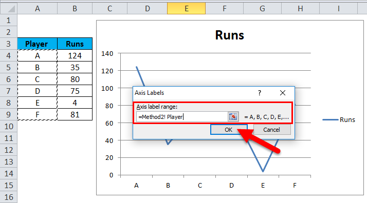
- Click on the Edit button from the horizontal category axis label.
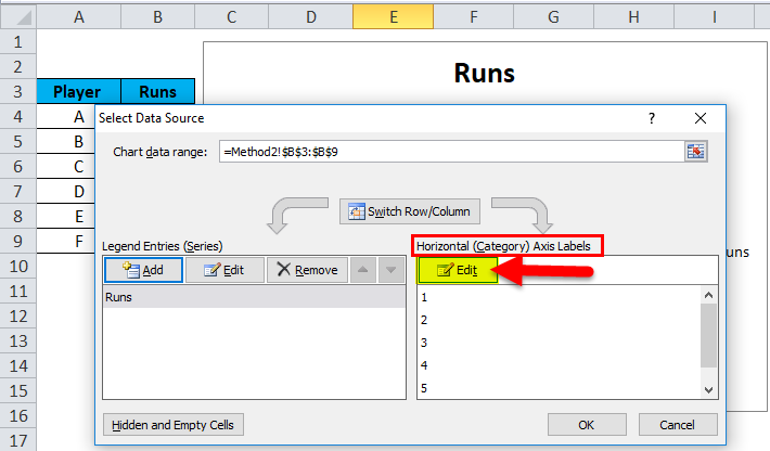
- In the axis labels, the dialogue box enters the worksheet name and named range (Method2! Player). Click OK.
- Give a Chart Title as Match Analysis.
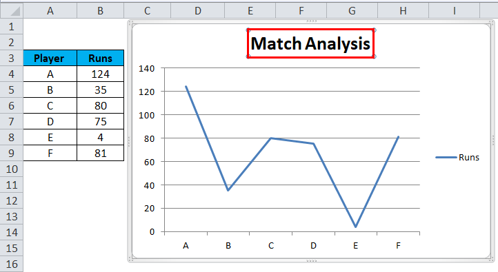
After following these steps, a dynamic chart is created by using the formula method, and also it will be updated automatically after inserting or deleting the data.
Pros of Dynamic Chart in Excel
- A dynamic chart is a time-efficient tool. Saves time in updating the chart automatically whenever new data is added to the existing data.
- Quick visualization of data is provided in case the existing data is customized.
- The OFFSET formula used overcomes the limitations seen with VLOOKUP in Excel.
- A dynamic chart is extremely helpful for a financial analyst who tracks companies’ data. Inserting the updated result helps them understand the company’s ratio trend and financial stability trend.
Cons of Dynamic Chart in Excel
- In the case of a few, hundreds of formulas used in the Excel workbook can affect the Microsoft Excel performance concerning the recalculation needed whenever the data is changed.
- Dynamic charts represent information more easily but also make more complicated aspects of the information less apparent.
- For a user not used to Excel, the user may find it difficult to understand the functionality of the process.
- Compared to the normal chart, dynamic chart processing is tedious and time-consuming.
Things to Remember About Dynamic Charts in Excel
- When creating name ranges for charts, there should not be any blank space in the table data or datasheet.
- Ensure to follow the naming convention, especially when creating a chart using name ranges.
- When using an Excel table as the first method, the chart will update automatically whenever the data gets deleted, but a blank space will appear on the right side of the chart. So, in this case, drag the blue mark at the bottom of the Excel table.
Recommended Articles
This has been a guide to Dynamic charts in Excel. Here we discuss its uses and how to create a Dynamic Chart in Excel with Excel examples and downloadable Excel templates. You may also look at these useful functions in Excel –
