Updated May 9, 2023
SUMIF Formula in Excel
In this article, we will learn about the SUMIF formula in Excel. We will also look into the use of the function with several examples.
The sum function adds cells or all cells in a range. The SUMIF function adds cells or ranges when a specific criterion is met. Thus, this function adds all the cells that fulfill a certain condition or criteria. A criterion could be a number, text, or logical operator. In short, it is a conditional sum of cells in a range.
This function is a worksheet function and is available in all versions of Microsoft Excel. It is categorized under Math & Trigonometry formulas.
The formula is written as below:
How to Use SUMIF Formula in Excel?
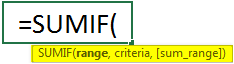
The syntax has arguments, as mentioned below:
- Range – It is a required argument. It is the cell range on which the condition/criteria are applied. The cell should contain numbers or text, dates, and cell references that have numbers. If the cell is blank, it will be ignored.
- Criteria – It is a required argument. It is the criteria that will decide which cells to be added. In other words, it is the condition based on which the cells will be summed up. The criteria can be text, number, dates in Excel format, cell references, or logical operators. It could be like 6, “yellow”, C12,” <5″, 05/12/2016, etc.
- Sum_ range – The cell range needs to be added. It is an optional argument. They are cells other than those found in range. If there is no sum range, the original cell range is added.
How to Use SUMIF Formula in Excel?
The SUMIF formula in Excel is very simple and easy to use. Let’s start with a very simple example of SUMIF. In this example, we only have one column or range.
Example #1
This is a very basic example with only two arguments.
Below is the single column data on which we will use SUMIF. We need to add cells that are above or >20 in the cell range A1: A8.
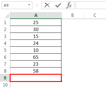
We will now write the formula in cell A9 as below:
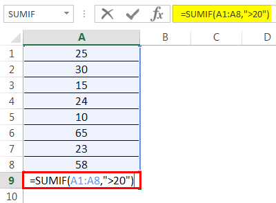
In this, the range is “A1: A8”, the criteria are “>20”, and then since there is no sum_range so the cells of range (A1: A8) will be added.
Press Enter to get the result.
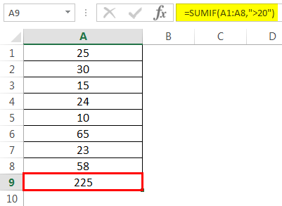
All cells above 20 are added in the range. Only cell A3 which has 15, and cell A5 which has 10, are excluded.
Also, we can use a cell reference as a criterion instead of hard-coding the actual value.
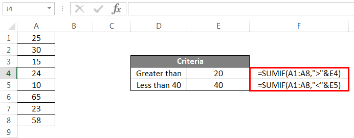
We have used E4 and E5 as cell references instead of 20 and 40. Now press Enter to see the result.
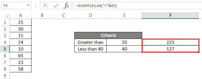
This is how we use cell references as criteria instead of writing them.
Example #2
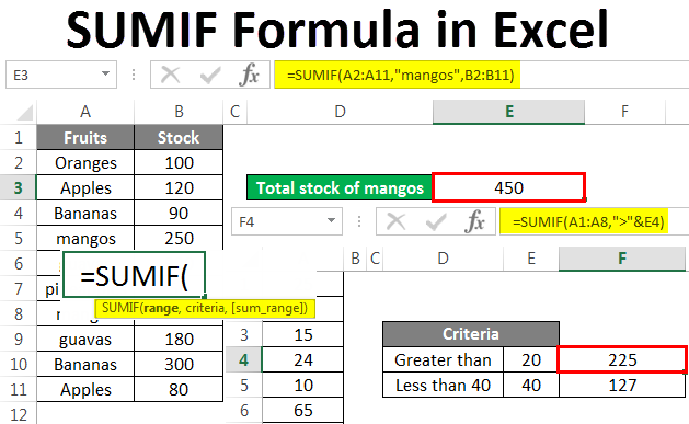
This example shows a data set of different fruits and their stocks, as shown below. Suppose we want to know the total stock of mangos out of all fruits.
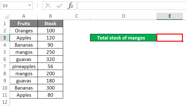
We will now write the formula in cell E3:
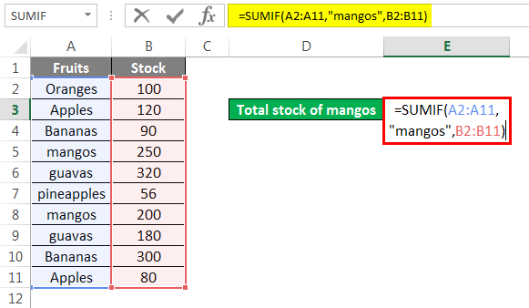
The arguments in the formula are explained below:
Range: A2: A11. In this range, the criteria of mangos will be applied.
Criteria: It is mangos, as we want to know the sum of mangos from all fruits.
Sum_range: The sum range here is B2: B11.
Press Enter to get the result.
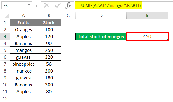
We have 450 mangos out of all fruits.
Example #3
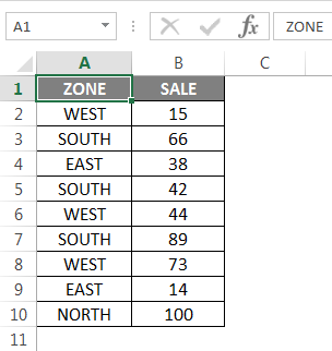
We have sales data from different zones. Let’s say we want to know the total sales for the South zone.
We will write the formula in cell B12 as below:
Range: A2: A10
Criteria: SOUTH
Sum_range: B2:B10
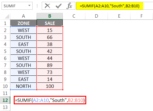
Press Enter.
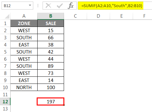
So the total sales for the south zone are 197. Also, we can use a cell reference in criteria instead of south.
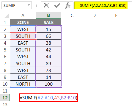
Here A3 is a cell reference used in place of “South”.Now press Enter.
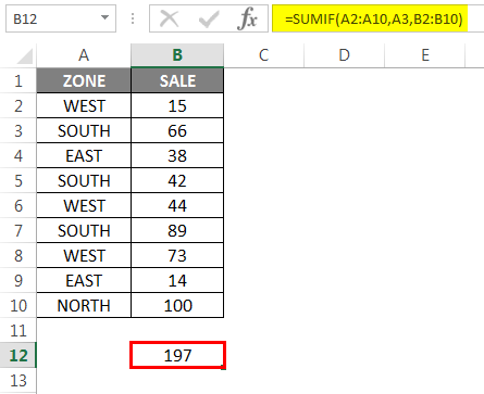
So we can also use cell references in place of writing the criteria.
Example #4
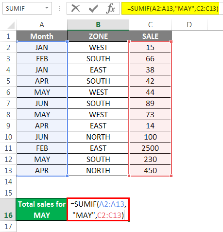
We have a sales data table for six months. And we want to find out the total sales for May.
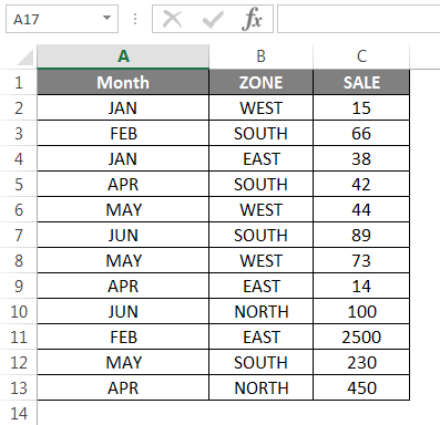
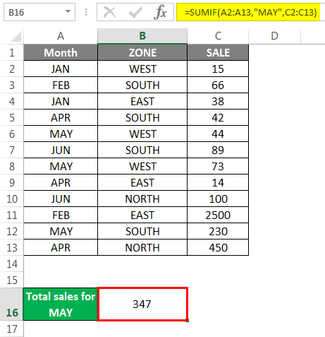
We will write the formula in cell B16.
Once you press Enter, you will see the Result.
We will now look at some different SUMIF scenarios with text criteria.
Example #5
We have sample data of balloons and their quantities.
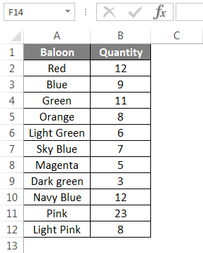
We want to sum up all blue balloons, whether sky blue or navy blue, out of all balloons.
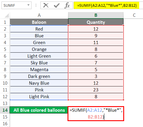
We will write the formula below:
Press Enter to get the result.
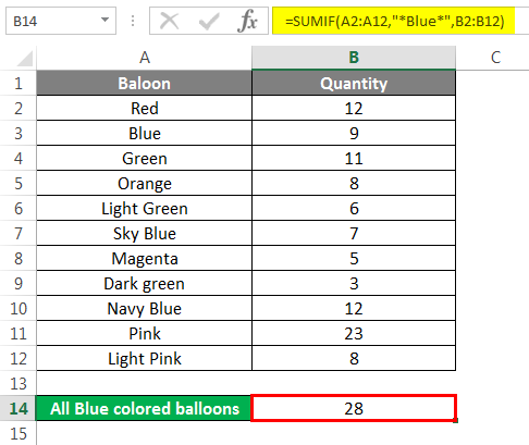
In this case, we want to sum the cell based on a partial match. Hence, all cells containing “Blue” will be summed up, single or combined with other words. So we use a wild card *.
And so Blue, sky blue, and navy blue are all summed up.
In case you want to add all balloons except for blue balloons. We will write the formula below.
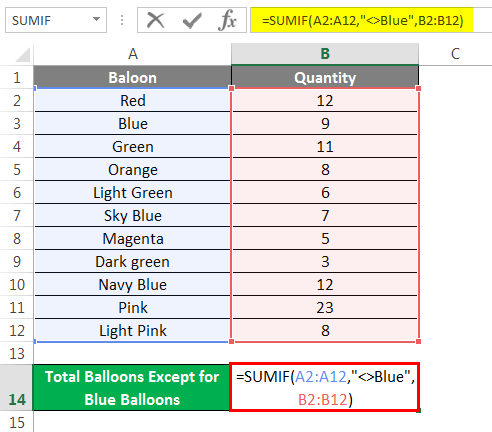
The criteria in this example are “<>Blue”, which means add all except for blue balloons. It will also add sky blue and navy blue in this case.
Press Enter to see the total number of balloons except for blue balloons.

We will write this formula if we want to add all balloons except for all shades of green.
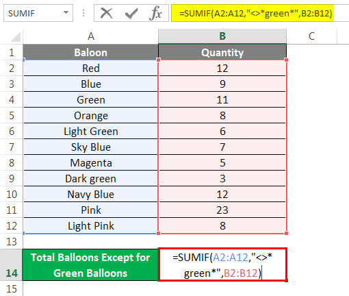
The criteria in this formula are any cell containing the word green or in combination with other words like dark or light green will not be summed up.
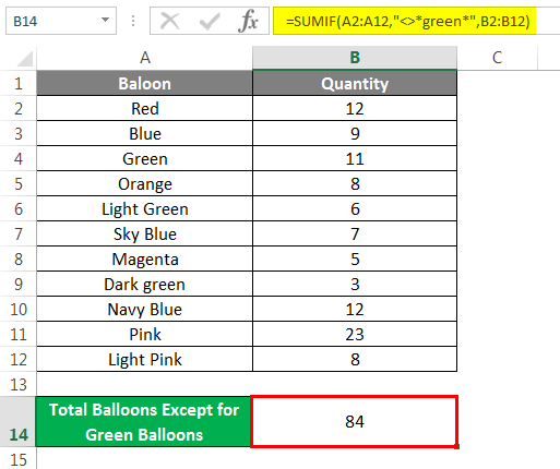
Hence, all balloons are summed up except for green, dark green, and light green balloons.
Also, we can use cell references in criteria when using logical operators.
Example #6
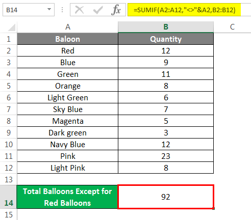
Taking our previous example, if we want to add all balloons except for red balloons.
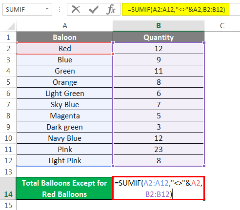
Press Enter to see the Result.
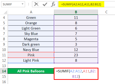
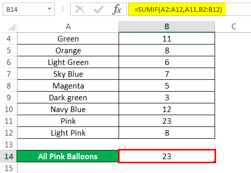
You can use the options below if you want only a specific cell or the “= to” operator. We will write the formula in any of the ways. Suppose we only need the sum of Pink balloons.
Or
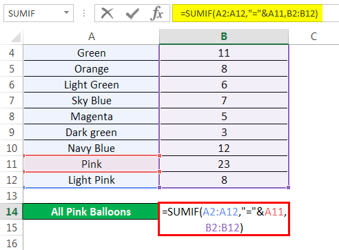
Both of them will give the below answer.
Let’s now see how to add blank cells using SUMIFs. Let us say we have the above data table with blank cells and want to sum up the blank cells. We can do so by writing the below formula.
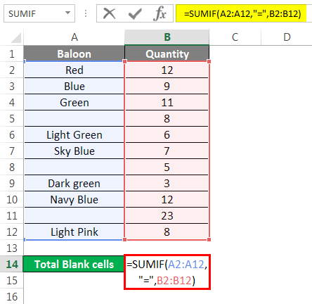
To see the sum of blank cells, press Enter.
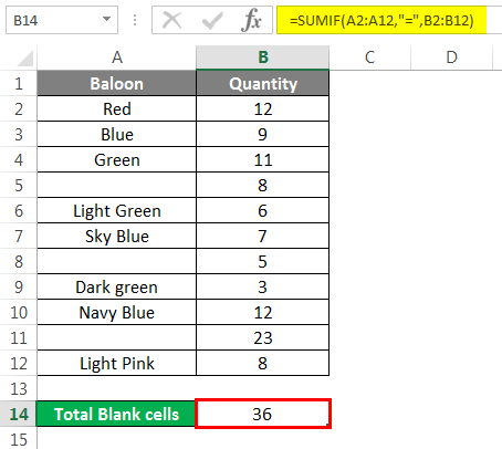
Here the logical operator “=” is used for blank cells. The above examples would have given you a clear understanding of the function and its uses.
Things to Remember
- To simplify things, make sure that range and sum_range are the same size.
- If the criteria are text, it should always be written within quotes.
- You might #VALUE! Error if the given text criteria are more than 255 characters.
- In SUMIF, the range and sum_range should always be ranges, not arrays.
- If you don’t provide a sum_range, the function will add cells within the range that meet your specified criteria.
Recommended Articles
This has been a guide to SUMIF Formula in Excel. We discuss using SUMIF Formula in Excel with examples and downloadable Excel templates. You may also look at these useful functions in Excel –
