Updated June 13, 2023
Pivot Table Formula in Excel
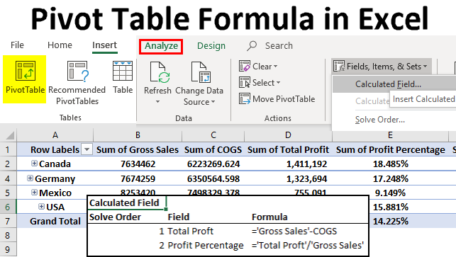
We can add and modify the formula available in default calculated fields in Excel once we create a pivot table. To see and update the pivot table formula, create a table with relevant fields we want to keep. After selecting or putting the cursor on it, select Calculated Fields from the drop-down list of Fields, Items & Sets from Analyze menu ribbon. We will see all the fields used in the pivot table along with the section Name and Formula section.
Custom Field to Calculate Profit Amount
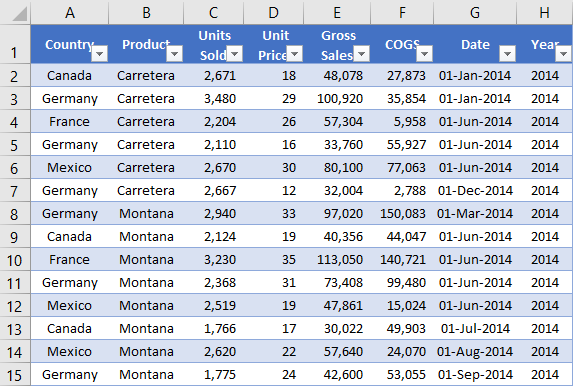
This is the most often used calculated field in the pivot table. Please look at the data below; I have the Country Name, Product Name, Units Sold, Unit Price, Gross Sales, COGS (Cost of Goods Sold), Date, and Year columns.
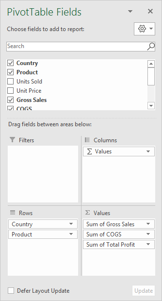
Let me apply the pivot table to find each country’s total sales and cost. Below is the pivot table for the above data.
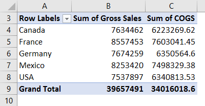
The problem is I don’t have a profit column in the source data. I need to find out the profit and profit percentage for each country. We can add these two columns to the pivot table itself.
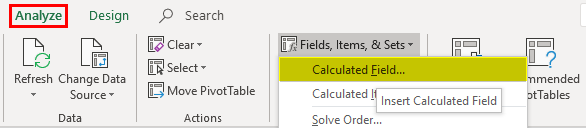
Step 1: Select a cell in the pivot table. Go to Analyze tab in the ribbon and select Fields, Items, & Sets. Under this, select Calculated Field.
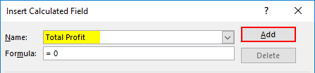
Step 2: Name your new calculated field in the dialog box below.
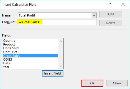
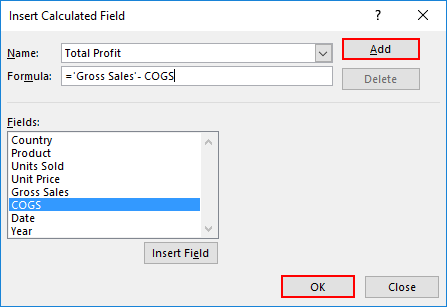
Step 3: In the Formula section, apply the formula to find the profit. The formula to find the Profit is Gross Sales – COGS.
Go inside the formula bar > Select Gross Sales from the below field and double click it will appear in the Formula bar.
Now type minus symbol ( – ) and select COGS > Double click.
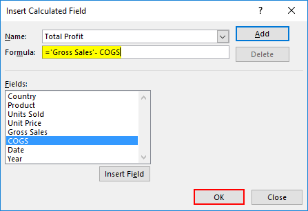
Step 4: Click on ADD and OK to complete the formula.
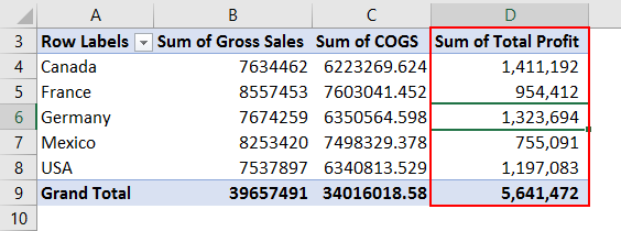
Step 5: Now, we have our TOTAL PROFIT Column in the pivot table.
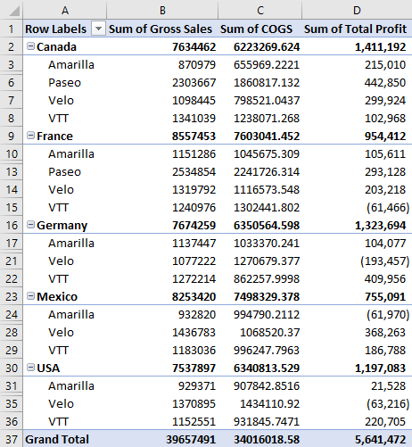
This calculated field is flexible, not limited to Country-wise analysis, but we can use this for all kinds of analysis. If I want to see the analysis country-wise and product-wise, I have to drag and drop the product column to the ROW field; it will show the breakup of profit for each product under each country.
Step 6: Now, we need to calculate the profit percentage. The formula to calculate the Profit Percentage is Total Profit / Gross Sales.
Go to Analyze and select Calculated Field under Fields, Items, & Sets again.
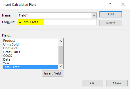
Step 7: Now, we must see the newly inserted calculated field Total Profit in the Fields list. Insert this field into the formula.
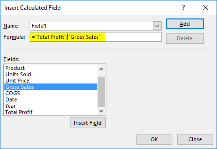
Step 8: Type divider symbol (/) and insert Gross Sales Field.
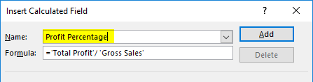
Step 9: Name this Calculated Field as Profit Percentage.
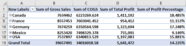
Step 10: Click on ADD and OK to complete the formula. We have Profit Percentage as the new column.
Advanced Formula in Calculated Field
Whatever I have shown now is the basic stuff of Calculated Field. This example will show you the advanced formulas in pivot table calculated fields. Now I want to calculate the incentive amount based on the profit percentage.
If the Profit % is >15% incentive should be 6% of the total profit.
If the Profit % is >10% incentive should be 5% of the total profit.
If the Profit % is <10% incentive should be 3% of the total profit.
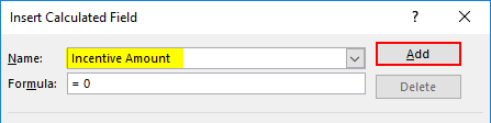
Step 1: Go to Calculated Field and open the below dialog box. Give the name as Incentive Amount.
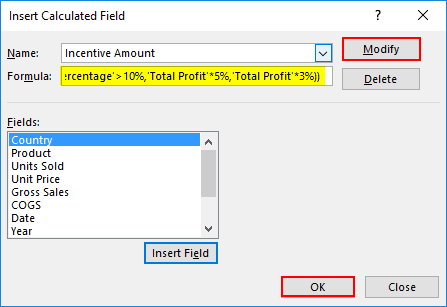
Step 2: Now, I will use the IF condition to calculate the incentive amount. Apply the below formulas as shown in the image.
=IF (‘ProfitPercentage’>15%, ‘TotalProft’*6%, IF(‘ProfitPercentage’>10%, ‘Total Proft’*5%, ‘Total Proft’ *3%))
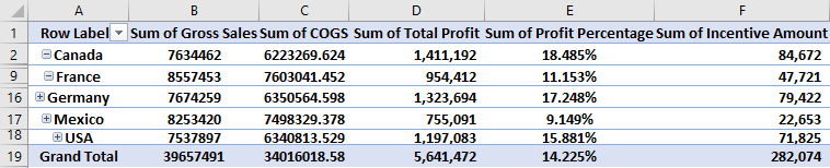
Step 3: Click on ADD & OK to complete. Now we have an Incentive Amount column.
Limitation of Calculated Field
We have seen the wonder of Calculated Fields, but it also has some limitations. Now look at the image below; if I want to see the breakup of the Product-wise Incentive amount, we will have the wrong SUB TOTAL & GRAND TOTAL of INCENTIVE AMOUNT.
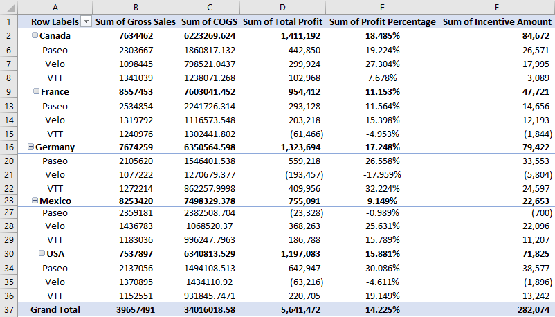
So be careful while showing the Subtotal of calculated fields. It will show you the wrong amounts.
Get a List of All the Calculated Field Formulas
If you do not know how many formulas are in the pivot table calculated field, you can get the summary of all these in a separate worksheet.
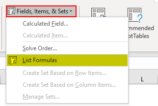
Go to Analyze > Fields, Items, & Sets –> List Formulas.
It will give you a summary of all the formulas in a new worksheet.
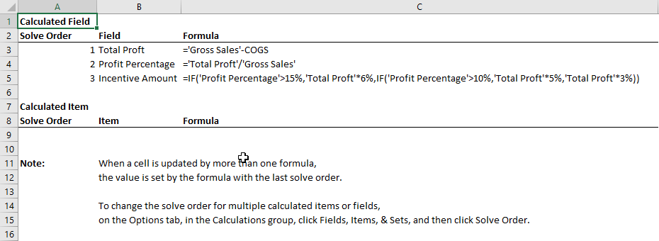
Things to Remember About Pivot Table Formula in Excel
- We can delete and modify all the calculated fields.
- We cannot use formulas like VLOOKUP, SUMIF, and many other ranges-involved formulas in calculated fields, i.e., all the formulas which require range cannot be used.
Recommended Articles
This has been a guide to Pivot Table Formula in Excel. Here we discussed the Steps to Use the Formula of the Pivot Table in Excel, Examples, and a downloadable Excel template. You may also look at these useful functions in Excel –
