Updated August 21, 2023
OR Formula in Excel
- MS Excel provides several logical inbuilt functions, one of which is the OR function, used to test multiple scenarios or conditions simultaneously. As it is a Logical function, it will only return True or False. Users can also use the OR Formula in Excel with other Logical functions, like AND, OR, XOR, etc.
- It will return true if any single argument or condition is true; else, it will return false. A user can test up to 255 arguments in the OR function.
Syntax of the ‘OR’ Function:
OR () – It will return a Boolean value, either true or false, depending on the argument provided inside the function.
The Argument in the Function:
- Logical1: It is a mandatory field, first condition, or logical value that a user wants to evaluate.
- Logical2: It is an optional field the user provides that he wants to compare or test with other conditions or logical values.
How to Use OR Formula in Excel?
OR Formula in Excel is very simple and easy. Let’s use the OR Formula in Excel with some examples.
Example 1
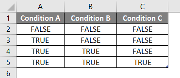
A user has A, B, and C conditions that he wants to evaluate in the OR function.
Let’s see how the ‘OR’ function can solve his problem of calculating.
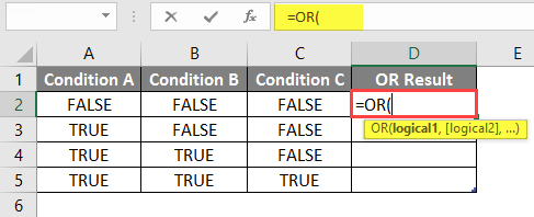
- Open MS Excel, Go to the Sheet where the user wants to execute his OR function.
- Create a Header Column with OR Result in the D column where we will execute the OR function.
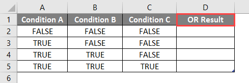
- Now apply the OR function in cell D2.
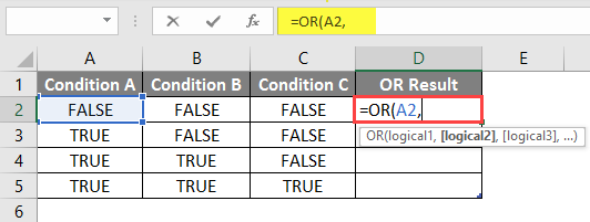
- Now it will ask for Logical1, which is available in the A column, then select the Value from the A2 cell.
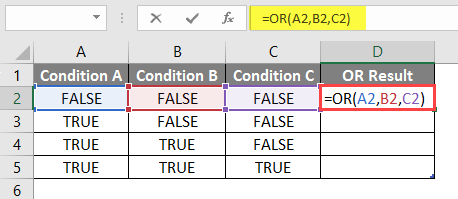
- Now it will ask for Logical2, Logical2, … which is available in the B and C columns.
- Select Value from the B2 and C2 cells.
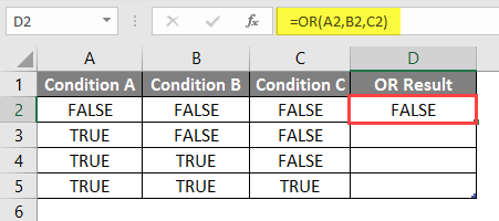
- Press on the Enter Button and the result is shown below.
- Now Apply the Same Formula to Other Cells by dragging the D2 formula until D5.
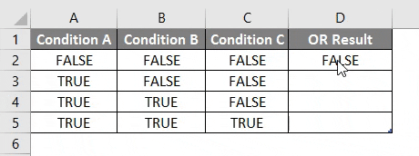
Summary of Example 1:
As the user wants to execute the OR function for different conditions, we have done in the above example.
As we can see, if a single condition is true, we are getting True as the OR output of rows 3 to 5. If all condition is false, then only we are getting false as OR output that is row no 2.
Example 2
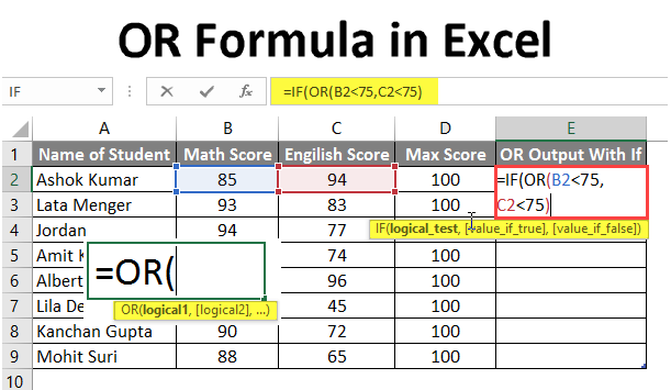
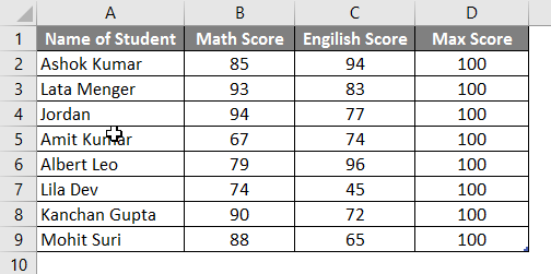
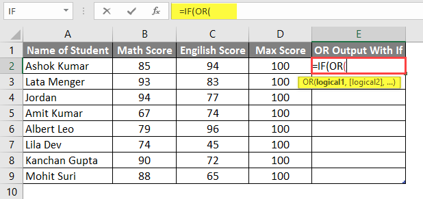
A User has a List of Student Score Card for Math and English, which he wants to evaluate for Pass and Fail, where he decides the minimum Score to Pass is 75 out of 100.
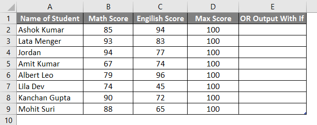
Let’s see how the ‘OR’ and ‘IF’ functions can solve this problem to evaluate the Fail or Pass status of the student.
- Open MS Excel, Go to the Sheet where the user wants to evaluate the Fail or Pass Status of the Student.
- Create a header column with ‘OR Output With If’ in column, E to execute the OR function.
- Now apply the IF Function in cell E2.
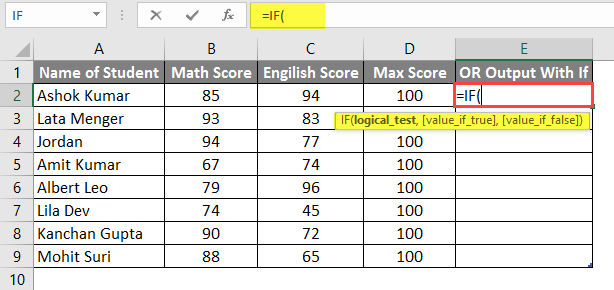
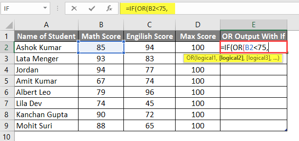
- Add OR Function to check if a student is scoring below 75 in any subject.
- Now it will ask for Logical1, a Math Score that needs to compare against a Passing Score of 75. So, just compare Math Score, available in the B column.
- Now it will ask for Logical1, Logical2, … which is an English score that must be compared against a passing score of 75. So, just compare the English Score, available in Column C.
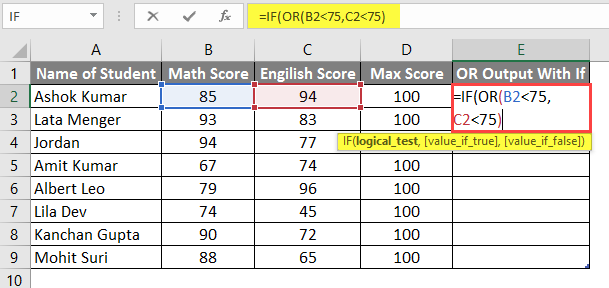
- It will then ask if the value is True, so if the student fails, his scores will be below 75 in any subject.
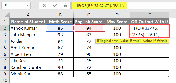
- Now it will ask if the value is False, and if the student passed, his scores would be above or equal to 75 in all subjects.
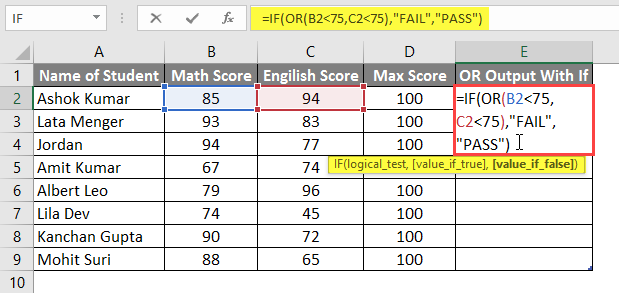
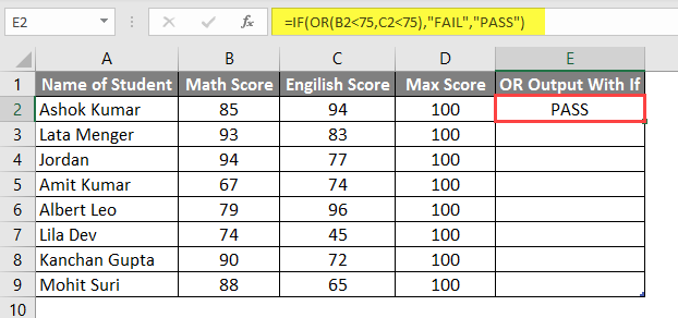
- Press the Enter Button and the result will be shown below.
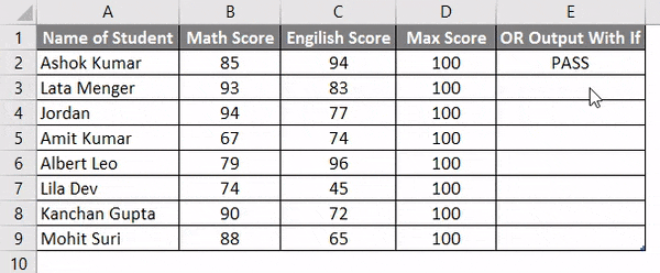
- Now apply the same Formula to other Cells by dragging the E2 formula to E9.
- To apply AND Formula with OR, we will create one Header in the F column and check if any student has passed in Math Science or English.
- Now apply AND & OR function to the G column.
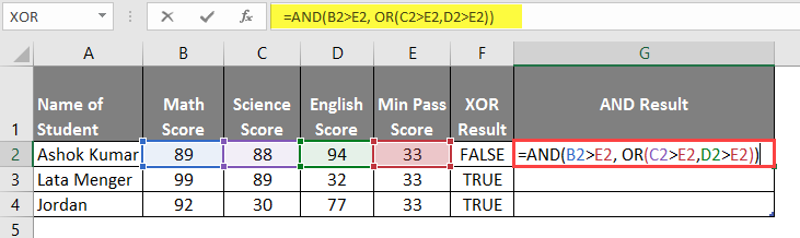
- After applying this formula, the result is shown below.
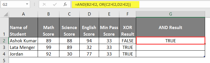
- Now apply the Same Formula to other Cells by dragging the G2 formula until G4.
Summary of Example 2:
As the user wants to execute the OR and IF function for different conditions, we have done in the above example.
As we can see, if a single condition is true, we are getting FAIL as the OR output of rows no 6, 8, 9, and 10. If all conditions are false, then only we get PASS as the OR output, that is, row no 3, 4, 5, and 7.
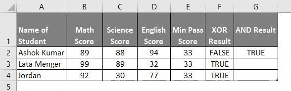
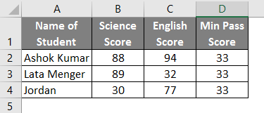
Example 3
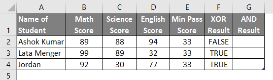
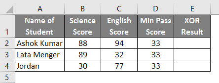
A user has a list of Student Score Cards for Science and English, which he wants to evaluate for FALSE and TRUE, where he decides the minimum pass score to pass is 33 out of 100.
Let’s see how the ‘XOR’ function can solve his calculation problem.
- Open MS Excel, and go to sheet3, where the user wants to execute his OR function.
- Create a header column with XOR Result in the E column where we will execute the XOR function.
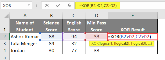
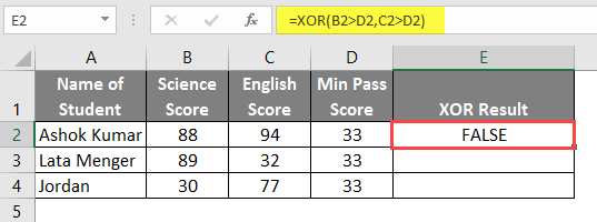
- Now apply the XOR function in cell E2.
- Press on the Enter Button and see the result below.
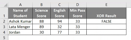
- Now apply the Same Formula to other Cells by dragging the E2 formula to E4.
Summary of Example 3: As the user wants to execute the XOR function for different conditions, we have done in the above example.
The XOR formula is Exclusive OR, where an odd number of conditions or True otherwise will always return False.
Things to Remember About OR Formula in Excel
- The OR function will return true if any argument or condition is true; otherwise, it will return false.
- A user can test up to 255 arguments in the OR function.
- If no logical value comes as an argument, it will throw an error #VALUE.
- A user can also use the OR function with other Logical functions, like AND, OR, XOR, etc.
Recommended Articles
This has been a guide to OR Formula in Excel. Here we discuss How to use OR Formula in Excel, practical examples, and a downloadable Excel template. You can also go through our other suggested articles –
