Updated July 4, 2023
What is the Pivot Table in Excel?
A Pivot Table in Excel summarizes large amounts of data by organizing the data into small conclusive tables. Pivot Tables can help create reports and charts to understand trends. It also allows data filters to view the details for areas of interest and explore more by changing the parameters.
It is known as a Pivot Table, letting the user rearrange the rows and columns around the data to arrive at the desired summary. Users can also view total sales for different products, show product sales in percentages, get employee headcount in different departments, etc.
For example, when we create Pivot Table for the data below,
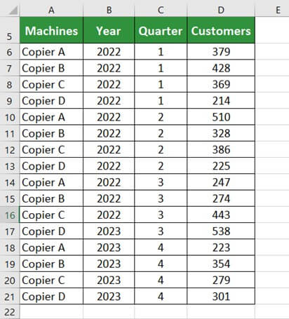
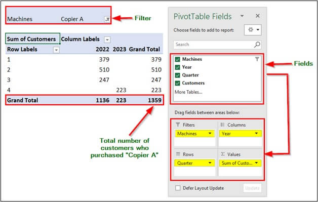
The data is organized in the below form:
Key Highlights
- Pivot Table in Excel helps complex group data in multiple ways to draw meaningful conclusions easily.
- We can rotate the data in the large data set to view it from different perspectives.
- We cannot add, subtract or modify data while creating a Pivot Table.
- We can use Pivot Tables for creating custom reports with appropriate formatting.
How to Create a Pivot Table in Excel?
Example #1
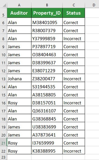
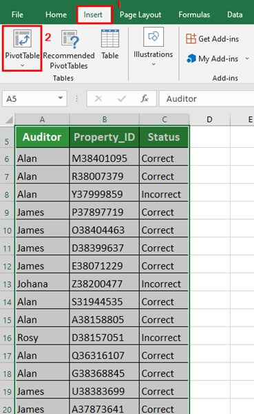
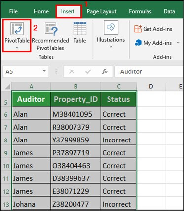
The table below shows a list of auditors with the properties they marked as correct and incorrect. Using the Pivot Table, we want to count the properties according to their status.
Solution:
Step 1: Select the data table and click on the Insert menu
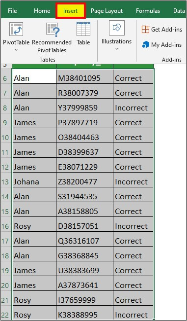
Step 2: Click on Pivot Table
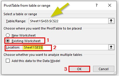
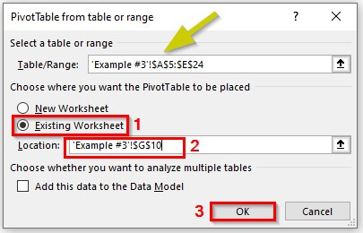
A dialogue box PivotTable from table or range is displayed as shown below
Explanation:
Table/Range is the selected data table.
Next, we must select whether we want the Pivot table in the New Worksheet or the Existing Worksheet.
Here, we select the Existing Worksheet.
Now, we have to specify the location (cell) for the Pivot Table. For this, click the desired cell, which will be displayed in the Location option in the dialogue box.
Now, click OK, and the below Pivot Table will be created.
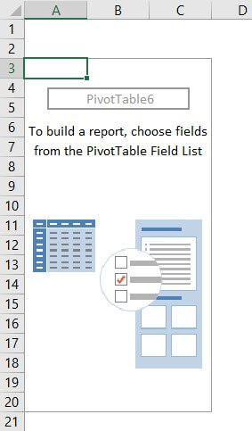
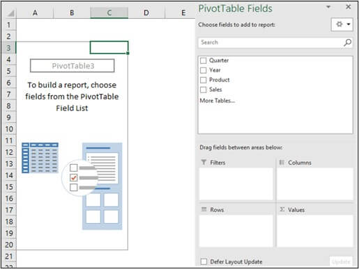
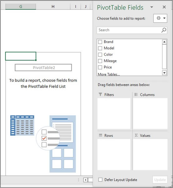
The above Pivot Table has no data. To enter data into it, click anywhere on the Pivot table, and we can see a Pivot Table Fields pane on the right side of the Excel Window, as shown below.
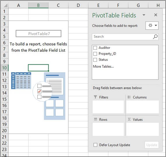
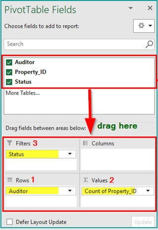
At the top, the Pivot Table lists fields (data table columns). At the bottom of the Pivot Table Fields pane are four areas (Rows, Values, Filters, and Columns) where we need to place the data fields.
- Rows: Data that is taken as a specifier
- Values: Count of the data
- Filters: Filters to select the desired data field
- Columns: Values under different conditions
We can place the data fields into the desired area by dragging them or clicking the checkbox next to the data field.
Step 3: Drag the Auditor field to the area Rows, Property_ID to Values, and Status to Filters.
The results are in the below table.
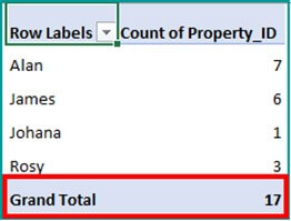
The table shows the Total count (17) of the Property_IDs checked by the auditors.
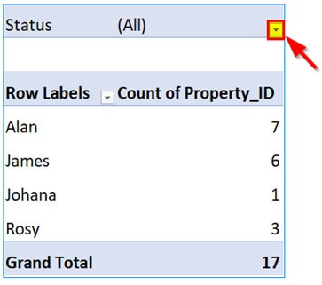
Now, we want to count the number of Property_IDs marked as Correct
Step 3: Click on the Filter section dropdown in the table
Step 4: Click on the Correct checkbox > Select Multiple Items > OK
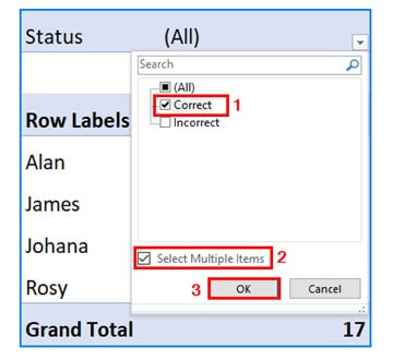
The result is displayed as shown below
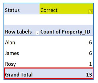
The above table shows the total number of Property IDs marked as correct to be 13.
Step 4: Select the Incorrect option from the filter (dropdown) to get the below result
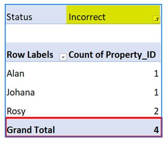
The above table shows the total count of Incorrect Property IDs.
Example #2
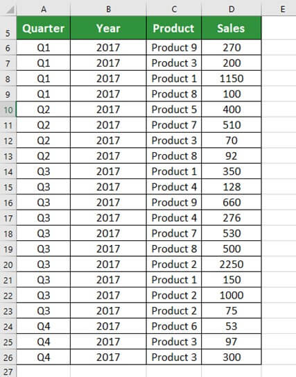
The table below shows sales of Product 1, Product 2, Product 3, Product 4, Product 5, Product 6, Product 7, Product 8, and Product 9 in the year 2017 in quarters- Q1, Q2, Q3, and Q4. We want to find the total sales of all the products using the Pivot Table.
Solution:
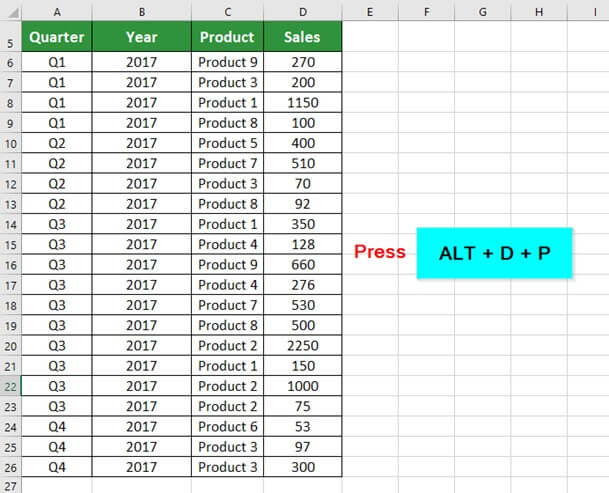
Here, we will use the alternative method to create the Pivot table. For that,
Step 1: Press the keys ALT + D + P on the keyboard
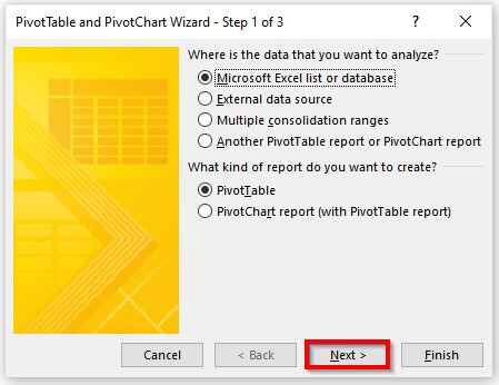
The PivotTable and PivotChart, Wizard dialogue box, open up. It asks two questions-
- Where is the data you want to analyze?
- What kind of report do you want to create?
Step 2: Select the first option for both questions, i.e.,
- Microsoft Excel list or database and
- PivotTable
And click Next.
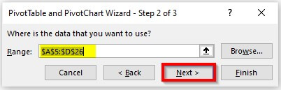
Now, Excel asks for a range of data. As we had already selected the data, therefore, it is prefilled.
Step 3: Click on Next
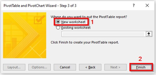
Now the dialog box asks us whether we want our pivot table in the same worksheet or a new worksheet. So,
Step 4: Select the New worksheet and click on Finish.
Now a Pivot Table is created with the PivotTable Fields pane on the right side of the Worksheet.
Step 5: Drag the field Quarter in the area Columns, Year in Filters, Product in Rows, and Sales in Values.
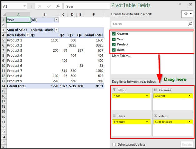
The Pivot Table is created as shown below
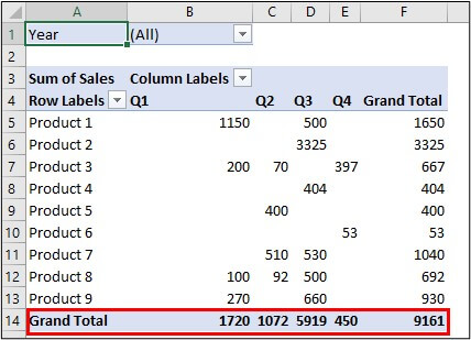
The above table shows the Total Sales of 9161.
Example #3
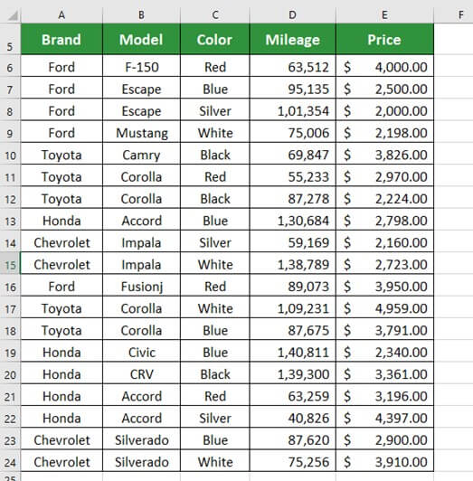
The below table shows a list of brands with their model, color, mileage, and price. We want to find the total price of all the Models of a Brand using the Pivot Table.
Solution:
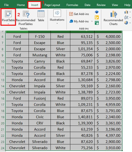
Step 1: Select the data table and click on Insert > Pivot Table
The Pivot table from the table or range dialogue box appears
Step 2: Choose Existing Worksheet, specify the location by clicking on the desired cell, and click OK.
The Pivot Table is created below with the Fields pane on the right.
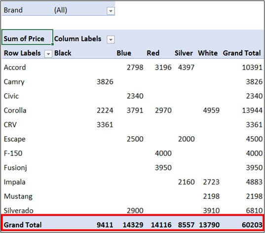
Step 3: Drag the field Brand in the area Filters, Model in Rows, Color in Columns, and Price in Values.

The Pivot Table is created below with a total price of $ 60203.
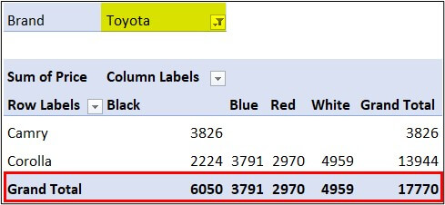
Step 4: Click the dropdown (filter) and select Toyota > Select Multiple Items > OK
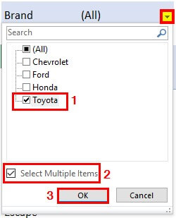
Excel creates a Pivot Table showing the total price ($ 17770) for all the models of Toyota.
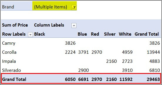
Now, we want to view the total price for Chevrolet and Toyota together
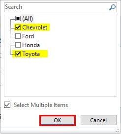
Click the dropdown (filter) and select Chevrolet and Toyota > Select Multiple Items > OK
Excel creates a Pivot Table showing the total price ($ 29463) for all the models of Chevrolet and Toyota
How to Move a Pivot Table in Excel?
To move a Pivot Table,
- Select the Pivot Table > PivotTable Analyze > Move PivotTable
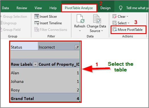
2. Specify the new location and click OK
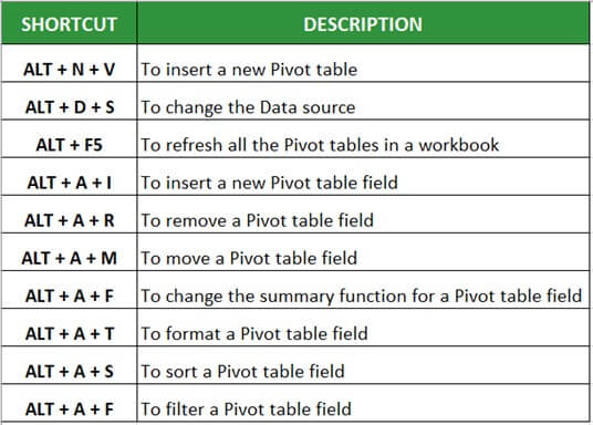
Shortcuts for Pivot table in Excel
Below are the shortcuts we can use while working with Pivot Table
Things to Remember
- Pivot tables do not change the values in the database.
- We can insert Pivot Tables in the same or a new worksheet.
- For convenience, we add pivot tables in a new worksheet.
- We can create Pivot tables with up to 500,000 records.
Frequently Asked Questions (FAQ)
Q1) Why use a Pivot Table in Excel?
Answer: Pivot Tables can track and analyze hundreds of thousands of data points with a compact table. We can use Pivot Tables to compare, highlight trends, or show relationships between parameters. Also, we can prepare multiple reports using the same Pivot Table.
Q2) Where is Pivot Table in Excel?
Answer: To locate the Pivot table,
Step 1: Select the data
Step 2: Click on Insert
Step 3: Select Pivot Table
Q3) Is there a limit to the number of rows in a Pivot Table in Excel?
Answer: A Pivot Table can display a maximum of 100,000 rows. Therefore, we cannot visualize more than 100k rows.
Q4) How many values can a Pivot Table handle?
Answer: Pivot tables can handle up to 1,048,576 items.
Q5) What are the disadvantages of a Pivot table in Excel?
Answer: The disadvantages of the Pivot table are:
- We cannot use the aggregate function with the Pivot table
- Pivot tables do not support conditional formatting.
- The Pivot Table does not work if there are blank rows or columns
Recommended Articles
The above article is a guide to creating a Pivot Table in Excel. For more such information, EDUCBA recommends the below-given articles.
