Updated August 19, 2023
Excel Logical Functions (Table of Contents)
Introduction to Logical Functions in Excel
There are various types of logical functions, some commonly used in Excel data operations. Logical functions in Excel work with conditions. They help deal with different situations accordingly. These functions perform work similar to IF-ELSEIF-ELSE statements in a programming language. These functions have simple syntaxes and can be beautifully combined with other functions to obtain desired results.
Types of Logical Functions in Excel
Excel’s various types of logical functions are IF, IFERROR, AND, OR, NOT, TRUE, and FALSE. In the following section, we will see how to use each through examples.
1. IF
A simple logical function checks whether to validate the condition as true or false. We will demonstrate the IF function using a very simple example. There’s a simple dataset containing data on students and their marks. Now, if the passing marks are 40, we would like to declare each student’s result in PASS and FAIL. This can be done using the IF function.
Syntax:
Example:
Step 1: When we enter the IF function, Excel automatically pops up the list of arguments, as shown in the following screenshot.
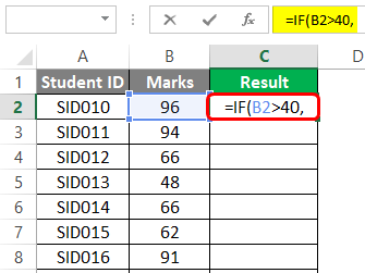
Step 2: The first argument is the logical test. In this case, the condition is that if marks are more than 40, then the result is PASS, or else it is FAIL. As shown below, we passed the condition as the argument in the IF function.
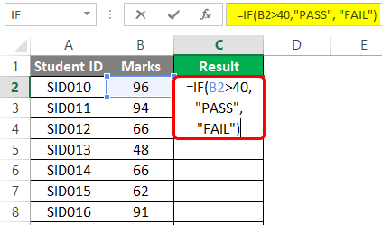
Step 3: The second and third arguments are ‘value_if_true’ and ‘value_if_false’. If marks exceed 40, the result should be PASS; otherwise, FAIL. This has been accomplished by passing the arguments shown in the following screenshot.
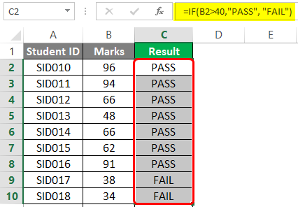
Step 4: Copy the IF function across all the required cells, and we returned the correct result as shown in the following screenshot.
2. IFERROR
There are various errors in Excel, and IFERROR uses to deal with these errors. Many times, in Excel, we are returned error values as results. In such cases, the IFERROR function becomes handy. We use this function when we want to return a meaningful result rather of an error.
Syntax:
As we can see in the syntax, the IFERROR function basically means that if the value passed into it is not an error value, then that value will be given as output by the function; otherwise, the value we specified in the ‘value if error’ argument.
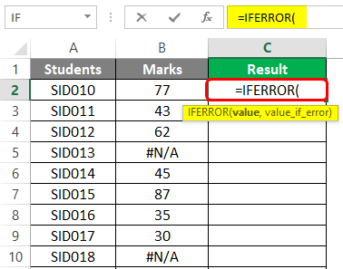
Step 1: The IFERROR function considers two arguments in the syntax. This is also shown in the screenshot below.
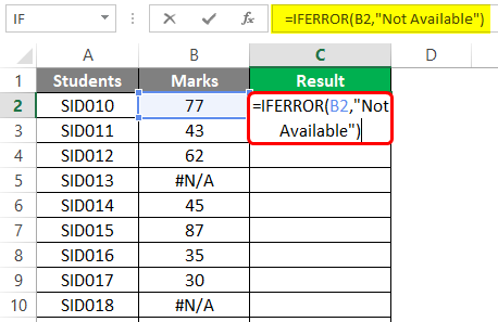
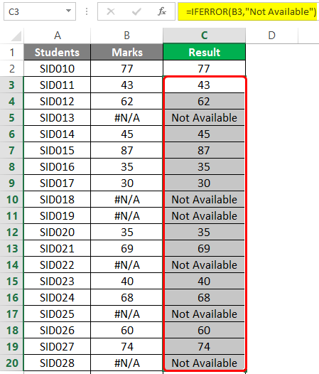
Step 2: In this example, we have marks for certain students. For some of the students, the result is not available, and for them, we have a #N/A error in the Marks column. We want this error value to be replaced with some meaningful text possible through IFERROR. The following screenshot shows this.
As we can see in the above screenshot, we passed marks as the first argument and kept the string “Not Available” as the second argument. It means if marks are valid, output marks or “Not Available”. This is shown in the following screenshot.
3. AND
This function returns either a TRUE or FALSE value by checking the conditions passed into it. If all the conditions passed into AND function are met, then the TRUE value is returned, and if even a single condition is not met, then the FALSE value is returned.
Syntax:
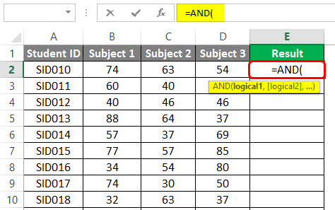
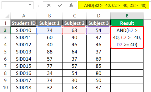
Step 1: We have marks for three different subjects for certain students. Now, we want to check if the student has passed or failed. If a student secures marks less than 40 even in a single subject out of the three subjects, he has failed the examination. We can determine the result for each student using the AND function. When we enter the AND function, we find that arguments are highlighted. In this case, they are logical conditions, as shown below.
Step 2: Using AND, we will get results for each student by passing the conditions in the function as shown below.
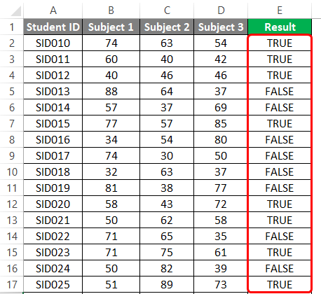
When the function is implemented, we get the result as shown below. Note, here, TRUE means pass, and FALSE means fail.
4. OR
It returns a TRUE value even if a single condition is met out of the total conditions passed. It returns FALSE when all the arguments are FALSE.
Syntax:
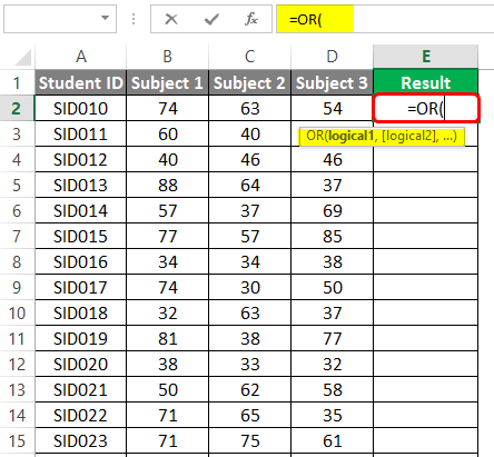
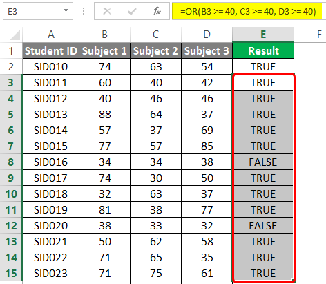
Step 1: We have marks for three different subjects for certain students. Now, if a student has secured 40 marks in at least one of the three subjects, the result should be a pass or a fail. When we enter the OR function, the arguments are highlighted below.
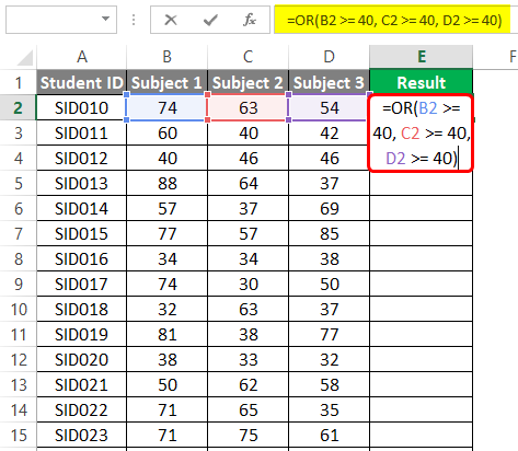
Step 2: The desired criteria for determining a student’s result can be met using the OR function below.
Following the above step, we get the desired result, as shown below. Observe it.
5. NOT
It reverses the logical value, i.e., TRUE to FALSE and FALSE to TRUE. It is usually implemented in context-based situations.
Syntax: NOT(logical)
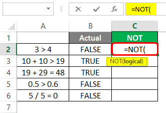
Step 1: We pass certain logical conditions into NOT and check how the function works. Have a look at the following screenshot.
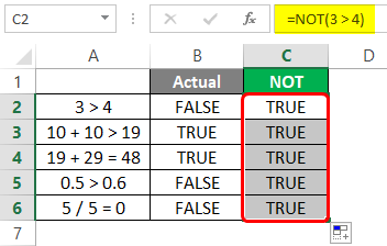
The actual result for each of them is shown. However, the logical values are reversed when we pass the logical conditions into the NOT function, as shown below.
6. TRUE and FALSE
They return corresponding logical values; TRUE returns TRUE, while FALSE returns FALSE.
Syntax: TRUE(), FALSE()
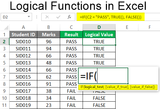
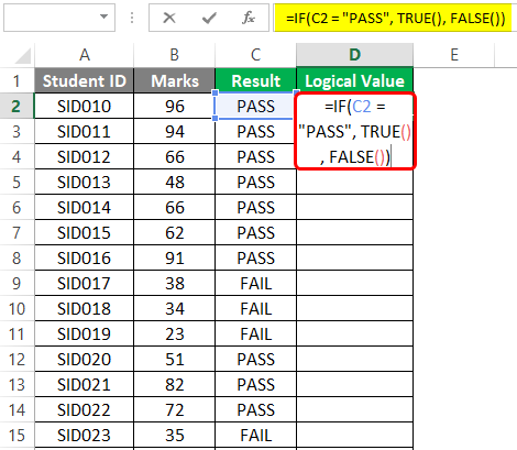
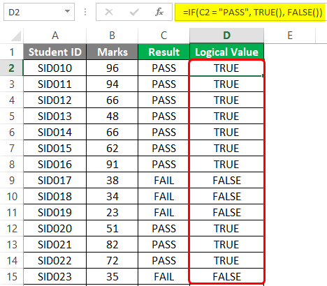
We have the result of the students. For PASS, we will display TRUE, and for FAIL, FALSE. The following screenshot shows the implementation.
The result that we obtained is shown below.
Things to Remember
- You should implement the logical functions in various contexts to understand their full capability.
- You should check the difference in available features in logical functions for different versions of Excel.
- Each argument in a logical function should be studied to understand its role and significance.
Recommended Articles
This has been a guide to Logical Functions in Excel. Here we discuss How to use Logical Functions in Excel, practical examples, and a downloadable Excel template. You can also go through our other suggested articles –
