Updated August 10, 2023
How to Match Data in Excel (Table of Contents)
Introduction to Match Data in Excel
Microsoft Excel offers various options to match and compare data, but we usually compare only one column in most scenarios. Comparing the data for one or more or multiple columns, various options are available based on the data structure. It’s the most frequent task use in comparative data analysis on tabular row or column data.
Definition of Match Data in Excel
It’s a process to find out or spot a difference between datasets of two or more columns or rows in a table. It can be done by various procedures, depending on the dataset structure type.
In Excel, we have a procedure or tool to track the differences between a row’s cells and highlight them, irrespective of the number of row or column datasets & worksheet size.
Examples of How to Match Data in Excel
Let’s check out the various available option to compare data sets between two rows or columns in Excel & to spot a difference between them.
Example #1
How to Compare or Match Data in the Same Row
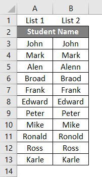
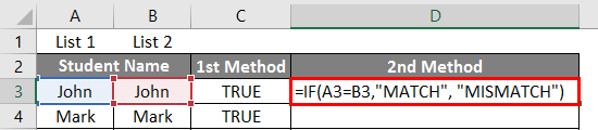
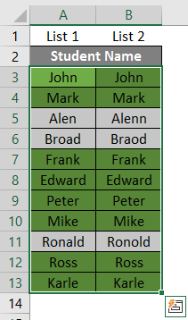
In the below-mentioned example, I have two columns, i.e., List 1 & 2, which contains the list of student names; now, I have to compare & match a dataset in these two columns row by row.
To check whether the name in List 1 is similar to list 2. There are various options available to carry out.
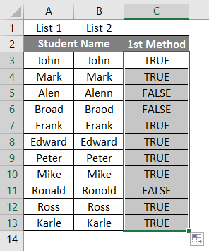
Method 1 – I can apply the below-mentioned formula in a separate column to check out the row data one by one, i.e., =A3=B3; it is applied to all the other cell ranges.
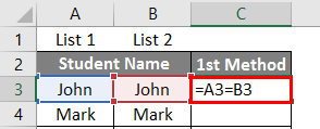
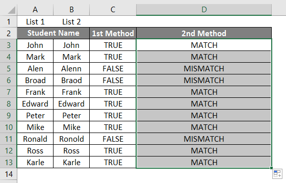
If there is a data match, it returns a value “True”; otherwise, it will return a “False” value.
Method 2 – To Compare data by using IF logical formula or test
If logical formula gives a better descriptive output, it compares case-sensitive data.
i.e., =IF (A3=B3, “MATCH”, “MISMATCH”)
Suppose the logical test is case-sensitive. It will help out whether the cells within a row contain the same content. I.e., Suppose the name is “John” in one row & “John” in the other row; it will consider it as different & result in Mismatch or a false value.
Here is the result mention below.
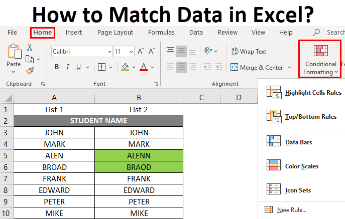
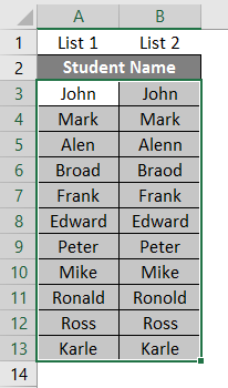
Method 3 – To Compare data with the help of Conditional Formatting
Here, suppose I want to highlight the matching data between two rows with some color, say, Green, otherwise no color for data mismatch; then, to perform this, Conditional Formatting is used with a set of certain criterion
- To perform conditional formatting, I must select the entire tabular data set.
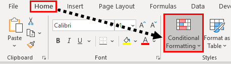
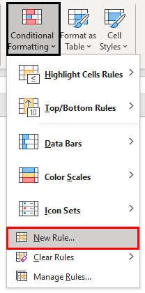
- Go to the Home tab, under the style option, and select a Conditional Formatting option.
- Various options under the conditional formatting appear in that select New Rule.
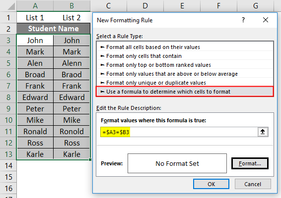
- Once you click on the new rule, the ‘New Formatting Rule’ dialog box appears; under the option to select a rule type at the top, you must select “Use a formula to determine which cells to format”. In the formula field, to compare & match a dataset between two rows, we need to enter the formula $A3 = $B3.
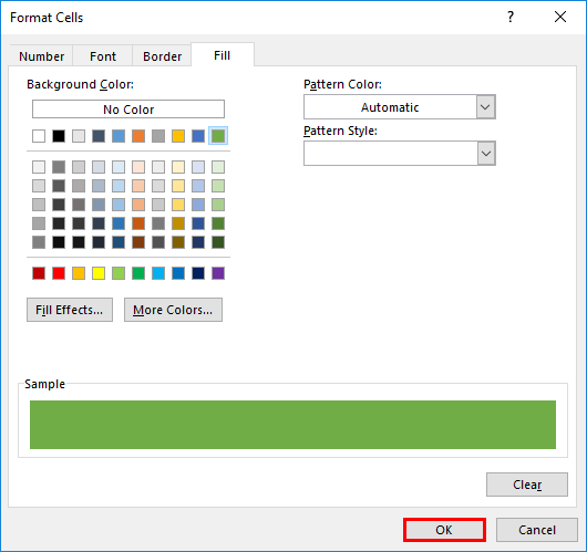
- Here, I want to highlight the matching data between two rows with green color, so in the format set option, I need to select a Green color and click on Ok.
- Again click on OK.
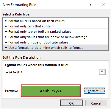
Now, it will highlight all the matching data with green color and no color for the data, which is a mismatch between rows.
You can use the above three methods to compare and match numeric data, date, or time values. The same process can use to compare multiple column data matches in the same row.
Example #2
How to Compare or Match Data between Columns & Highlighting the Difference in the Data
In some cases, the dataset matches may be in different rows (It is not present in the same row); in these scenarios, we have to compare two columns & match the data.
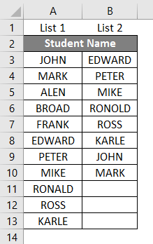
In the below-mentioned example, student list 1 in column B is slightly bigger than student list 2 in column C. and. Also, a few names are there in both student lists, but it is not present in the same row (such as John, Mark, and Edward).
Data match or comparison between two columns can be made through a duplicate option under conditional formatting.
Let’s check out the steps involved in carrying out this procedure.
- To perform conditional formatting, I must select the entire tabular data set.
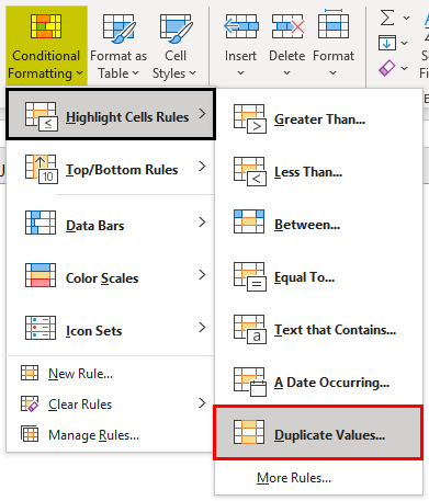
- In the Home tab, select a Conditional Formatting option under the style option.
- Various options under the conditional formatting appear; under the Highlight Cells Rules, you have to select the Duplicate Values.
- Once the duplicate values are selected, a popup message appears, where you need to select the color of your choice to highlight the duplicate values; here, I have selected Light Red Fill with Dark Red Text.
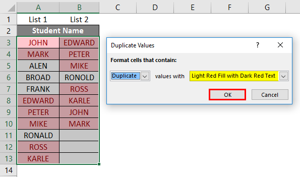
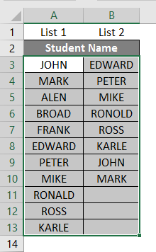
After selecting, you can observe that common students present in both columns are highlighted with red color (along with dark red text), while the unique values are not colored.
Example #3
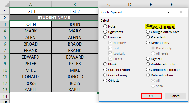
Highlighting the Row Difference with the help of the “Go to Special” Feature
Compared to other methods, with the help of this option, we can perform the task faster. It can also use for multiple columns.
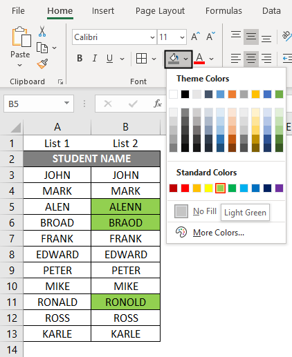
- To perform “Go to Special“, you need to select the entire tabular data set and click on CTRL + G; once it is selected, the Go-To Special dialog box appears; in that, you need to select “Row Difference” and then click on OK.
- It will highlight the cells with different datasets; now, you can color it green to track a difference in the dataset between rows.
Things to Remember about the Data Match in Excel
Apart from the above methods, various third-party add-on tools perform the textual data match in Excel.
Fuzzy Lookup Add-In tool for Excel
It is most commonly used to match and compare a customer’s name & address data. It will help track the difference in the data table within a selected row. It will also help find various errors, including abbreviations, synonyms, spelling mistakes, and missing or added data.
Recommended Articles
This is a guide on How to Match Data in Excel. Here we discuss How to Match Data in Excel using different methods, Different Examples, and a downloadable Excel template. You may also look at the following articles to learn more –
