Updated June 8, 2023
Introduction to Match Multiple Criteria in Excel
In this article, we will learn about Excel Match Multiple Criteria. As a data analyst, you must always meet multiple criteria and conditions to get the desired result. In Excel, you can use the IF Statement for conditional outputs. However, sometimes you must construct more sophisticated logical tests to get the desired results. It may include multiple IF Statements (i.e., nested IF) or some logical operators under IF statements. Ideally, we can construct multiple criteria using the logical AND & OR operator under the IF Statement.
- AND Operator: If you use logical AND operator/keyword under IF Statement, you will get TRUE if all conditions/criteria are satisfied. Otherwise, it will return FALSE.
- OR Operator: If you use logical OR operator/keyword under the IF statement, you’ll get TRUE if at least one of the multiple conditions/criteria are satisfied. Else it will return FALSE.
How to Match Multiple Criteria in Excel?
To Match Multiple Criteria in Excel is very simple and easy. Let’s understand this function with some examples.
Example #1 – AND/OR Operators Works for Multiple Criteria
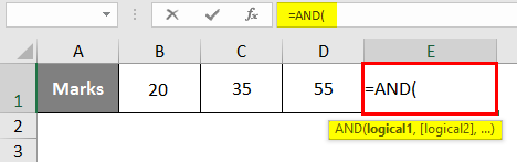
Suppose we have three sets of marks for a student, as shown below:

Step 1: In cell E1, as we need to check how AND operator works for multiple criteria, start initiating the formula by typing “=AND(
Step 2: We need to specify logical criteria under AND function. Use criteria as cell value greater than 16 for all cells (B1, C1, D1). You can use a comma as a separator to separate the multiple criteria conditions. See the screenshot below:
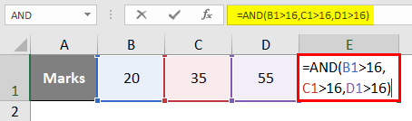
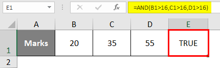
Once you press Enter key, you can see TRUE as a result in cell E1. Because all values in cells B1, C1, and D1 are greater than 16, resulting in a TRUE Boolean output.
Step 3: Change the value in cell B1 to 12 and see the result in cell E1.
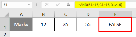
You can see the same criteria under AND function. If we change the value under cell B1 to less than the criteria value (i.e., 16), we will get the output as FALSE. Since the value in cell B1 is not greater than 16.
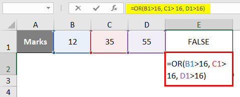
Step 4: In cell E2, use the OR to check how it works; use the same criteria values. Ideally, OR gives Boolean output as TRUE if at least one of the criteria is satisfied.
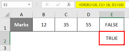
Press Enter key to see the output as TRUE in cell E2 since C1 and D1 have values greater than 16. However, with E1, it is still FALSE since all the conditions are not satisfied.
Example #2 – Complex Criteria in Combination with IF, AND/OR
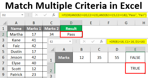
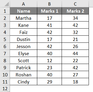
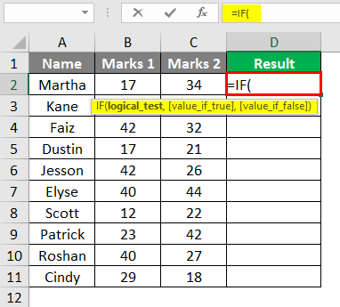
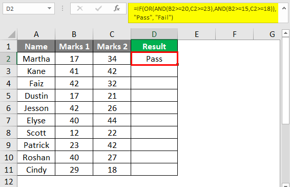
Suppose we conduct two tests in a class of 10 students and have Marked in both tests for each student stored under columns Marks 1 and 2, respectively. We wanted to check whether the student had passed the exam or not. See the screenshot of the below data.
To check whether the student has passed the test or failed, we can combine IF statements with AND/OR operator to combine the multiple criteria.
Suppose we have two criteria under this example:
Criteria 1: Column B >= 20 and Column C >= 23
Criteria 2: Column B >= 15 and Column C >= 18
If it meets the criterion, the student will Pass; otherwise, he/she will fail. Let’s figure out this tricky criterion with IF, AND, OR.
Step 1: In cell D2, initiate the formula for IF Statement by typing “=IF(
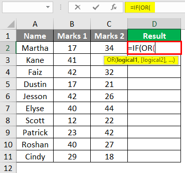
Step 2: Initiate an OR condition within the IF statement as shown below:
Step 3: Now, we must add two AND conditions within this OR condition separated by a comma. Use (AND(B2>= 20, C2>=23), AND(B2>=15, C2>=18)) under OR condition within IF Statement and close the bracket for OR condition.
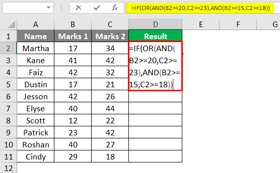
This condition will first check if Marks 1 and 2 are greater than or equal to 20 and 23, respectively (first AND condition) OR if not. It will check whether Marks 1 and 2 are greater than or equal to 15 and 18 (second AND condition). The student will be considered a Pass if at least one of these conditions meets the criteria; otherwise, the student will be considered a Fail.
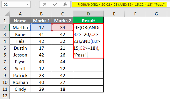
Step 4: Add the [value_if_true] as “Pass” under the formula in cell D2 to specify that if at least one condition gets satisfied, a student is a pass.
Step 5: Add “Fail” as a value for [value_if_false] under the IF statement to complete the formula and close the brackets to complete it. Press Enter key to see the output in cell D2 whether the student named “Martha” has passed the exam or not.
Step 6: Drag the formula across cells D2:D11 to have a result value, either Pass or Fail, for all the students named in column A. Select D2:D11 and press Ctrl + D as a keyboard shortcut to copy the formula across rows.
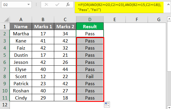
This is how we can match multiple criteria under Excel with the help of IF statement, AND & OR logical operators. This article ends here. Let’s conclude with some key points to remember.
Things to Remember
- You can use logical operators such as AND, OR, and conditional statement IF to match multiple criteria under Excel.
- Microsoft Excel tests all the conditions under AND even if the previous condition appears FALSE. This is a bit unusual as in other programming languages. If the previously checked condition is FALSE under logical AND, the system stops checking other subsequent conditions.
- If all the conditions satisfy in logical AND, it will return TRUE. Otherwise, it returns as FALSE.
- The logical OR operator returns TRUE if at least one of the conditions meets the criteria or else FALSE.
Recommended Article
This has been a guide to Excel Match Multiple Criteria. Here we discuss how to Match Multiple Criteria, practical examples, and a downloadable Excel template. You can also go through our other suggested articles –
