Google Sheet Formulas – Introduction
Google Sheets formulas are a fundamental tool for working with and analyzing data in Google Sheets. These formulas help us perform calculations & statistical analysis, manipulate data, and automate tasks in Google Sheets.
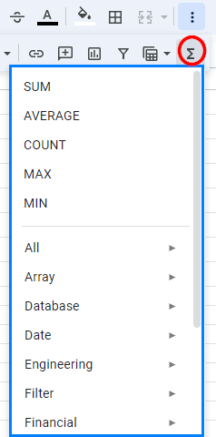
Using the functions option in the toolbar, you can find all Google Sheets formulas and functions (array, database, logical, math, etc.). The functions option is present at the right end of the toolbar.
How to Use Google Sheets Formulas?
To use Google Sheets formulas, follow these steps:
- Select a cell and start typing an equals sign (=).
For example, select cell A1 and type =. - Then, you can either type the entire function name or select a function from the drop-down menu that appears as you type.
For example, type like this: =AVERAGE - Type an open parentheses, add arguments (data or cell references), and then close the function with a closing parenthesis.
For example, it should look like this: =AVERAGE(A2:A10) - Press Enter to calculate the result.
- If you want to apply the formula to other cells, Sheets will show an option to auto-fill the rest of the cells. You can also copy and paste formulas as needed.
Example
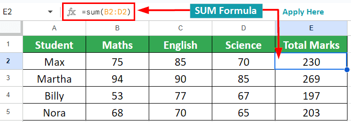
Suppose you need to find the total marks for each student, you can use this SUM formula:
Top Google Sheet Formulas List
Here are some common and frequently used Google Sheets formulas:
Let’s see how to use the above functions with the help of some examples:
1. SUM Formula
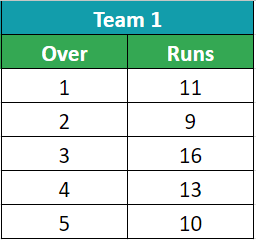
In a Cricket match, Team 1 has completed 5 overs and wants to find out their total runs scored to set a target for Team 2. You can find it by using SUM Formula in Google Sheets.
Given:
Solution:
In cell B7, add the SUM formula: =sum(B2:B6) and hit Enter.
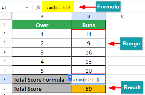
The SUM formula will give you a total of 59 runs. Therefore, Team 2 needed to score 60 runs to win the match.
2. AVERAGE Formula
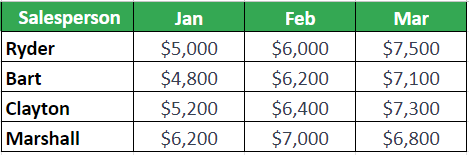
Suppose you are managing a sales team and want to calculate the average sales for each salesperson over a quarter. You can find it by using the AVERAGE formula.
Given:
Solution:
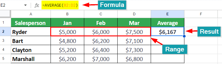
In our example, we will first find the average sale of Ryder.
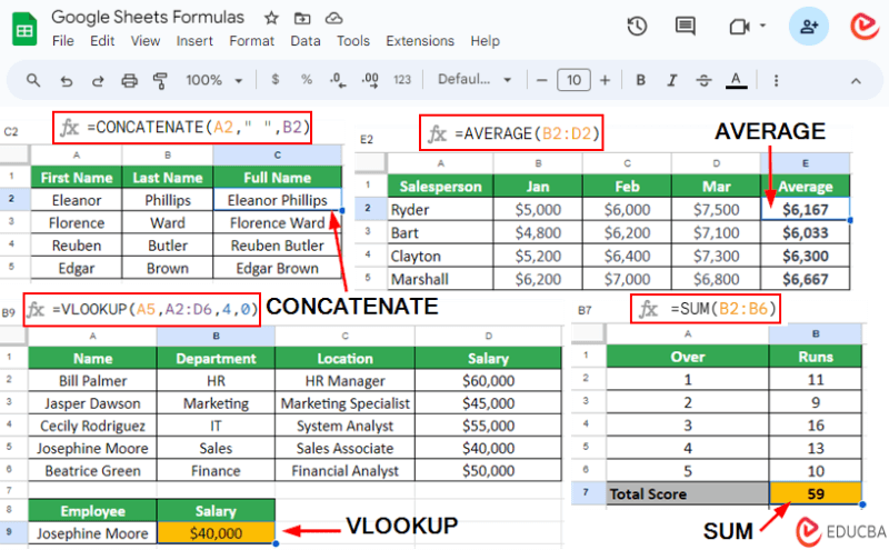
To do so, select cell “E2” and enter formula: =AVERAGE(B2:D2)
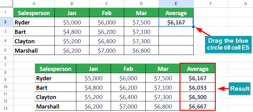
To find the average sale of other members, drag the blue circle to cell “E5,” as shown below:
3. MAX Formula
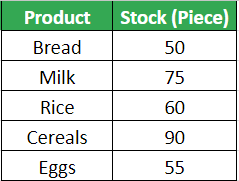
Suppose you are managing inventory for a grocery store and want to find out which product has the highest stock level. For this, you can use the MAX formula.
Given:

Solution:
To find the maximum number of stock, select cell “B7” and type formula: =MAX(B2:B6)
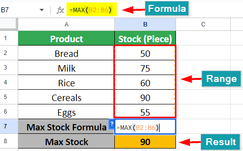
The maximum stock is of Cereals, i.e., 90 pieces.
4. MIN Formula
Let’s use the example we used for the MAX function, but now we will find the minimum stock level for a product using the MIN function.
Given:
Solution:
To find the minimum number of stock, select cell “B7” and type formula: =MIN(B2:B6)
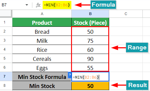
The minimum stock is of Bread, i.e., 50 pieces.
5. IF Formula
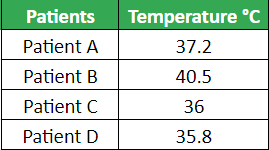
We have patients’ body temperature data and want to find which patients have a fever. We want to display “Fever” for those who have a fever (temperature above 38°C) and “No Fever” for others (temperature below 38°C).
Given:
Solution:
Select cell “C2” and type the formula: =IF(B2>38,“Fever”,“No Fever”).
If the patient’s body temperature exceeds 38°C, the formula will show “Fever” and vice versa.
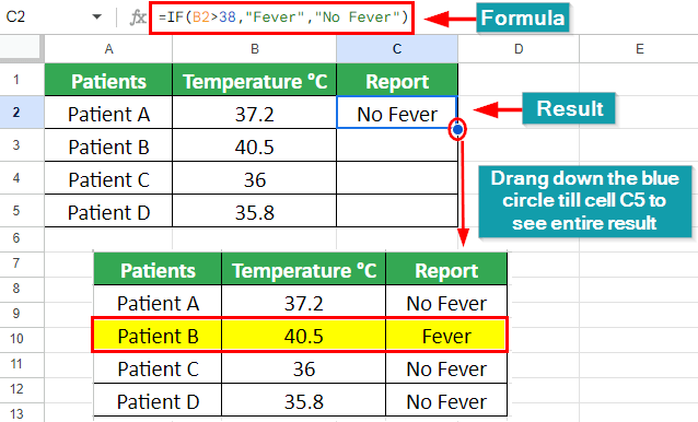
As a result, we can see that Patient B is having a fever of 40.5 °C.
6. VLOOKUP Formula
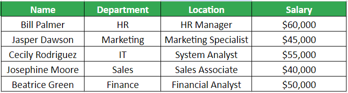
We have employee data and want to find the salary of Josephine Moore. Instead of manually finding it, we can use the VLOOKUP formula in Google Sheets.
Given:
Solution:
We are looking for the salary of “Josephine Moore,” so we have entered her name in cell A9. And we will find the result in cell B9 by using this formula: =VLOOKUP(A5,A2:D6,4,0)
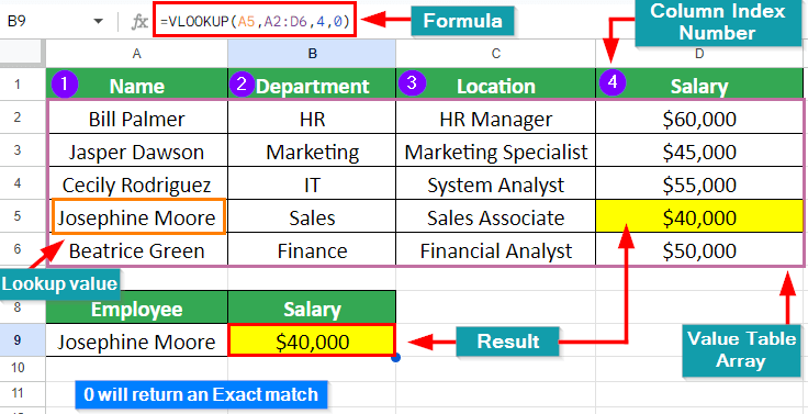
As a result, the salary of Josephine Moore is $40,000.
7. HLOOKUP Formula
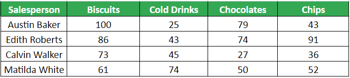
We have sales data with salespersons and the number of products they have sold. We want to find out how many chocolates Calvin Walker has sold. To do so, we will use the HLOOKUP formula.
Given:
Solution:
We have entered Calvin Walker’s name in cell A8. And we will find the result in cell B8 by using this formula: =HLOOKUP(D1,A1:E5,4,0)
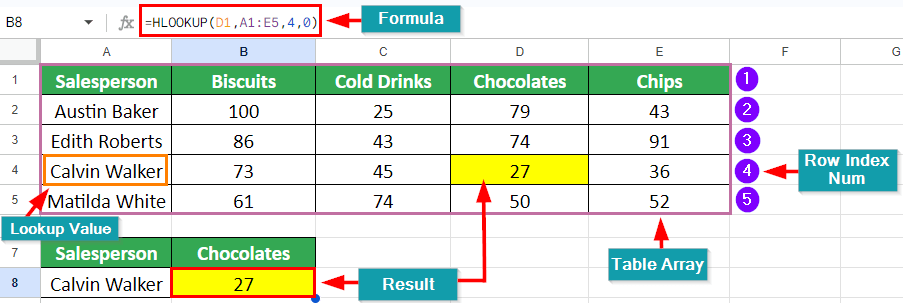
As a result, Calvin Walker has sold 27 chocolates.
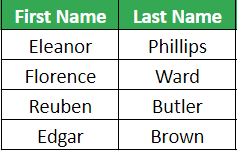
8. CONCATENATE Formula
We have a table in which first and last names are in two different columns. We want the full name to appear in one cell. To do so, we can use the CONCATENATE formula.
Given:
Solution:
Select cell “C2” and type formula: =CONCATENATE(A2,” “,B2), hit enter, and drag down the blue circle till cell “C5” as shown below:
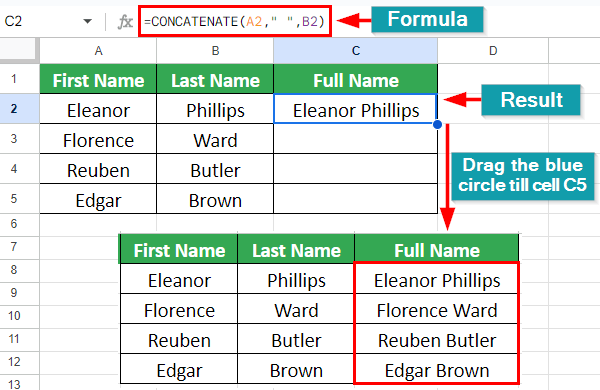
As a result, it gives its full name in one cell with a space between them.
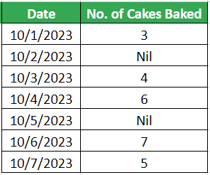
9. COUNT Formula
Suppose Adam bakes cakes at home for business and wants to know how many days a week he has baked cakes. He can use the COUNT formula in Google Sheets to count the number of days.
Given:
Solution:
Select the cell “B10” where you want to show the result and type formula: =COUNT(B2:B8)
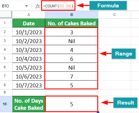
As a result, we can see that Adam has baked 5 days in a week.
10. COUNTA Formula
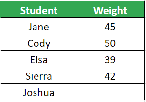
Suppose we have a list of students with their weight. We want to calculate how many students have done their weight check. To do this, we can use the COUNTA formula in Google Sheets.
Given:
Solution:
Select cell “B9” and type the formula: =COUNTA(B2:B6)
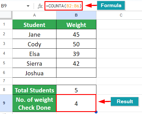
As a result, we can see that 4 students have done their weight check, and one is remaining.
11. IFERROR Formula
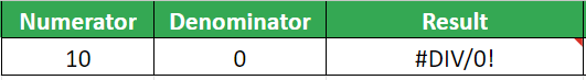
Let’s say we have a division formula, and we want to avoid the #DIV/0! error that occurs when dividing by zero by displaying a custom message in such cases. To do so, we can use the IFERROR formula.
Given:
Solution:
Select the cell D2 and enter “=IFERROR(A2/B2, “Cannot divide by zero”)” as the formula.
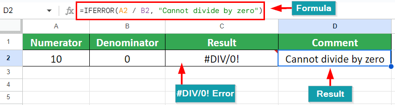
As a result, the IFERROR formula will display “Cannot divide by zero” if a division by zero error occurs.
12. DATE Formula
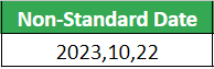
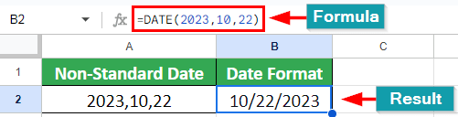
Suppose we have dates in a non-standard format and need to convert them into the correct date format. We can use the DATE formula in Google Sheets.
Given:
Solution:
Select cell “B2” and type the formula: =DATE(2023,10,22)
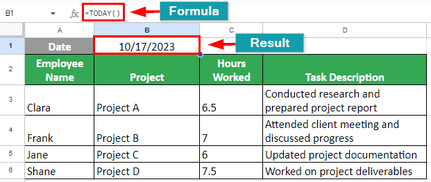
13. TODAY Formula
Suppose we want a cell to automatically display the current date, ensuring that it updates to the current date every day. This can be done by using the TODAY function.
Given:
Solution:
Select cell “B1” and enter the formula: =TODAY()
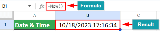
14. NOW Formula
Zara is working on a Google Sheet, and before adding any data, she has to add the current date and time. To do this, she can use the NOW formula.
Solution:
Select the cell “B1” and type the formula: =Now()
15. LEN Formula
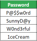
Let’s say your company has a policy that requires passwords to be at least 8 characters long. You can use the LEN formula in a cell to suggest a password meeting this requirement.
Given:
Solution:
Select cell “B2” and type the formula: =LEN(A2) and hit enter.
Drag the blue circle till cell “B5” to the full result of all passwords.
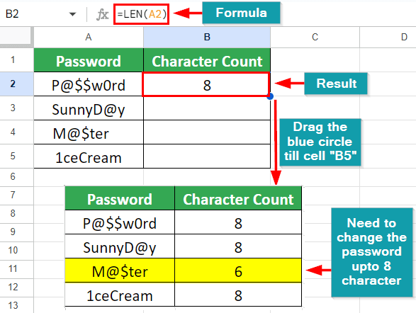
As a result, we can see that one password is less than the limit. Hence, we need to change it and make it up to 8 characters.
Recommended Articles
We hope this article on Google Sheets Formulas was beneficial to you. For more related articles, check the following,
