Updated August 22, 2023
Writing Formula in Excel
What would be your answer when I ask you, “What is Excel?” A tool that helps to store, slice, and dice the data plus a tool that can help us calculate sums, percentages, interest rates, etc., right? The most essential as well as an important part of Excel is a formula.
The formula is nothing but an equation that allows you to perform various calculations under Microsoft Excel. These formulae are the easiest way of calculation based on the given data.
However, being new to Excel, you might not always be able to handle the Excel formulae. It is very easy and simple, though, to add formulae under Excel. This article will try to teach you how to Write Formulas in Excel, and you will be master in applying the same after going through this article.
Let’s see how we can create/write a formula under Excel.
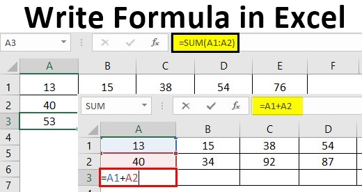
First, every Excel formula starts with the equals sign (‘=’) inside an Excel cell. After this sign, you can write the equation in which you want Excel to perform calculations or any inbuilt function name (Ex. SUM), which performs a calculation and returns the output in a given cell.
How to Write Formula in Excel?
Let’s understand How to Write the formula in Excel with a few examples.
Example #1
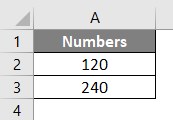
Step 1: Suppose we have two numbers, 120 and 240, in cells A1 and A2, respectively, in the Excel sheet. See the screenshot below:
Now, I want to add these two numbers; We’ll see how this can be achieved.
Step 2: In cell A4, start typing the equation by simply using equals to sign and then using 120 + 240 to add these two values. See the screenshot below for a better understanding.
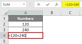
Step 3: Press Enter Key to see the result. You can see 360 as a result of cell A4, as shown below.
This is how a basic formula can be entered under Microsoft Excel. What if we change the numbers in cells A1 and A2 to different values? Will the formula under cell A3 change values? Well, let’s see by doing so.
Step 4: Change the numbers in cells A1 and A2 to 120 and 240, respectively.

If you check cell A3, it still shows the result for old values (i.e. 120 + 140 = 360). Because in cell A3, we have used the equation 120 + 140. These are values that are fixed and not dynamic ones. Therefore, to eliminate such a situation, Excel also provides an option to use dynamic ranges under an equation/formula for that sake.
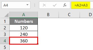
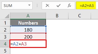
Step 5: In cell A3, tweak the formula to =A2+ A3. What we tried doing here is, instead of giving a number as an argument, we supplied the cells containing a number as an argument. This will be beneficial when you change the numbers in cells A2 and A3; values in cell A4 will automatically change after performing the operations. This is how making your formula dynamic using a range of cells works.
After using the above formula, the output is shown below:
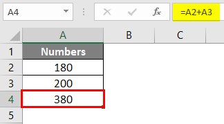
If I change the values under cells A1 and A2, the results in cell A3 will automatically change. See the screenshot below.

Example #2
Excel has a more user-friendly approach when it comes to applying the formula. You just can simply copy-paste the formula from one cell to another by dragging it through. Let’s see how to do it.
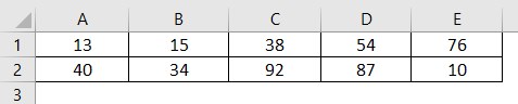
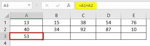
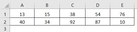
Suppose we have data as shown below across the first and second rows of different columns (A to E), and we wanted to get a sum for each column in their third row, respectively. We’ll see how Excel works in this situation.
Step 1: In cell A3, create an equation using a dynamic range of cells that sums the values under A1 and A2. You can use =A1+A2 as a formula under cell A3 to get the sum of the numbers within those cells.
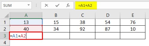
Also, Press Enter key to see the output in cell A3.
Step 2: Now, select cell A3 and then drag the formula across A3 to E3 to apply the same formula that sums up each column’s first and second rows. You should get the output as shown in the screenshot below:
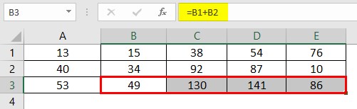
Well, you have multiple ways to achieve this result. You can select the entire third row across columns A to E and just press Ctrl + R to copy and paste the formula under cell A3 to other columns. Or else, you can copy the formula under cell A3 by Ctrl + C and paste it one by one in each B3, C3, D3, and E3 to achieve the same result.
Example #3
In this example, we will work on using the built-in Excel functions. How to use the built-in Excel function to perform a task (ex., Summing numbers across the rows).
Consider the same data as shown in example 2, and we wanted to have the sum of the first two rows of each column within the third row. However, we will use a built-in Excel function named SUM to achieve this result this time.
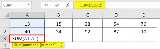
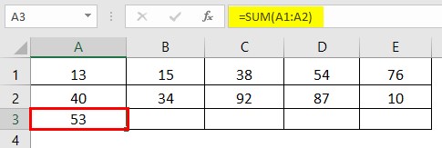
Step 1: In cell A3, start typing =SUM; a list of all functions containing SUM as a keyword will pop up. Select the SUM function through that list by double-clicking on it.

Step 2: Select the range of cells A1 to A2 using your computer mouse or laptop touchpad as an argument to the SUM function. Because these are the cells that we wanted to sum up.
You can also use the comma to separate the values instead of these ranges.
Step 3: Complete this formula by adding closing parentheses at the end of this function and press the Enter key to get the sum of cells A1 and A2 under cell A3.
This function precedes the equation in Example 2 by a huge margin when we have tons of data. Ex. Consider you have 5 Lacs Excel Rows, and you wanted to sum those up. You would not like to input each cell reference for 5 Lacs of time, would you?
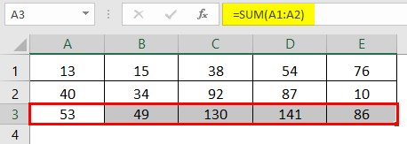
Step 4: You can drag this formula across the different columns for the same row, use Ctrl + R to populate it across all the rows, or copy and paste it one by one to each column. The choice is all yours. You’ll get the final output as shown below:
This is it from this article. Let’s wrap things up with some points to be remembered:
Things to Remember About Write Formula in Excel
- To use a formula in Excel, you need to start it with equals to sign. You also can start a formula with a Plus or minus sign.
- You can have different operational formulae for subtraction, multiplication, division, squaring a number, etc. However, all these operations are better done with built-in Excel functions because these functions precede operational formulae.
Recommended Articles
This is a guide to Writing Formulas in Excel. Here we discuss How to use Write Formula in Excel, practical examples, and a downloadable Excel template. You can also go through our other suggested articles –