Updated June 9, 2023
TIME in Excel
Excel’s time function is just another function that returns HHMM AM/PM Format time. We just need to feed Hour, Minute, and Second as per our requirement, and the time function will return the same value in AM and PM details. We need to note that if the Hours’ range is less than and equal to 12, then the time we get would be in AM and post 12; the time would be in PM till 11:59 in the clock.
TIME Formula in Excel:
The Formula for the TIME Function in Excel is given below.
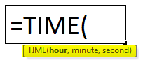
Arguments:
- Hour: If the hour value exceeds 23, it will be divided by 24, and the remainder will be used as the hour value. This means that TIME(24,0,0) is equal to TIME(0,0,0), and TIME(25,0,0) is equal to TIME(1,0,0).
- Minute: If the minute value exceeds 59, then every 60 minutes will add 1 hour to the hour value. This means that TIME(0,60,0) is equal to TIME(1,0,0), and TIME(0,120,0) is equal to TIME(2,0,0).
- Second: If the second value is greater than 59, then every 60 seconds will add 1 minute to the minute value. This means that TIME(0,0,60) is equal to TIME(0,1,0) and TIME(0,0,120) is equal to TIME(0,2,0)
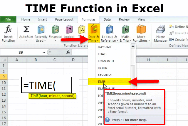
Steps to Open TIME Function in Excel
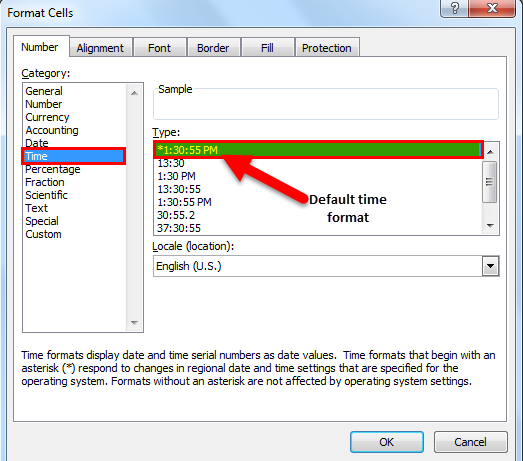
We can enter the time in a normal format so that Excel takes the default one. Please follow the below step by step procedure. Choose the time format in the Format Cells dialog; you may have noticed that one of the formats begins with an asterisk (*). This is the default time format in your Excel.
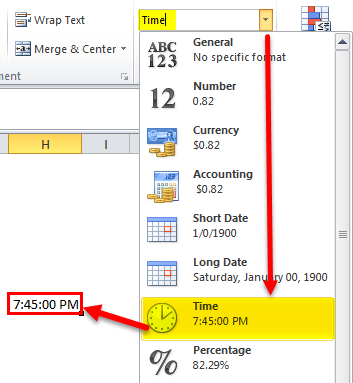
To quickly apply the default Excel time format to the selected cell or a range of cells, click the drop-down arrow in the Number group on the Home tab and select Time.
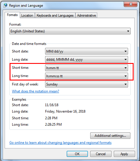
To change the default time format, go to the Control Panel and click Region and Language. If your Control panel opens in Category view, click Clock, Language, and Region > Region and Language > Change the date, time, or number format.
How to Use the TIME Function in Excel?
This TIME Function in Excel is very simple and easy to use. Let us now see how to use the TIME Function in Excel with the help of some examples.
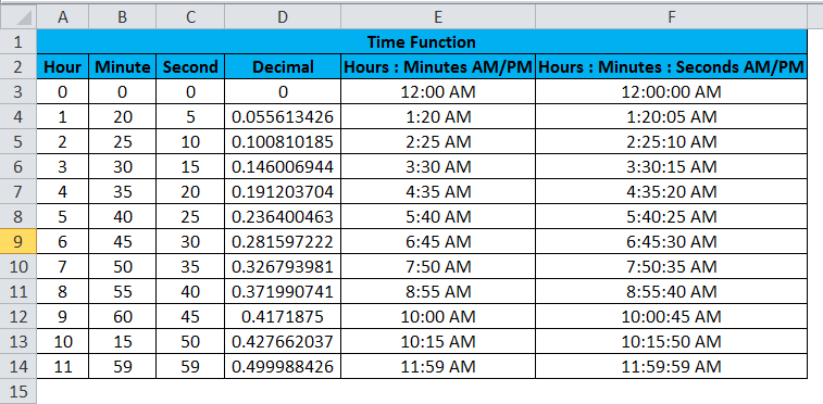
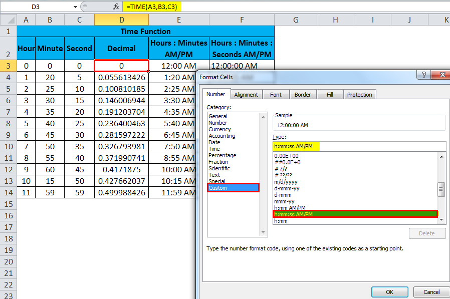
In the above example, we have three columns Decimal, Hours: Minutes, Hours: Minutes: Seconds, with three different formats which show the TIME function result.
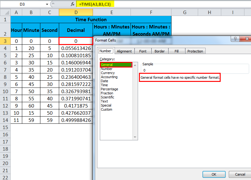
Decimal
We used the same TIME Function in this format and displayed the General (Decimal) format. To convert into a decimal format, right-click, choose format cells, and then choose general.
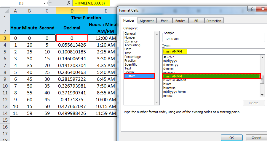
Hours: Minutes
The second format we have used is Hours & Minutes; to display in the above format, right-click and choose the format cell. There, we will find the custom option where we will get various hours formats to choose the appropriate format for H: MM AM/PM.
Hours: Minutes: Seconds:
The third format is Hours: Minutes: Seconds, where we have used the same TIME function to display it. To create a right-click and choose format cell, we will find the custom option where we will get a variety of hours formats to choose the appropriate format for H:M: SS AM/PM.
This time function can be useful in all productivity scenarios. Remember that the TIME function will “roll over” back to zero when values exceed 24 hours, wherein the advanced MOD function can be exactly used to differentiate AM/PM. This MOD function will take care of the negative numbers problem. MOD will “flip” negative values to the required positive values.
For example, if the employee works for 9 hours and he extends his Overtime for another 5 hours. In this scenario, if we want to find the start and end times, we can use the MOD function to calculate how many hours an employee has worked.
What is MOD Function?
The MOD function “Returns the remainder after a number is divided by a divisor.”
The Formula for MOD Function:
=MOD(number, divisor)
Calculating the date and time difference in Excel is a common task. Unfortunately, depending on the requirements, it is also not always simple.
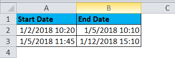
In the example below, column A contains a start date and time, and column B an end date and time. We wish to calculate the elapsed time in days, hours, and minutes, e.g., 11 days, 4 hours 9 minutes.
There are multiple ways of calculating the date and time difference in Excel. In this scenario, we will need to get a little clever. As you may know, date and time values are stored as numbers in Excel. For example, the 05/01/2018 10:10 is stored as 2.993055556.
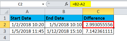
Therefore, if I write the formula as =B2-A2.
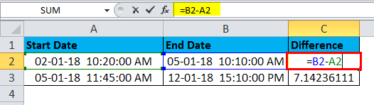
Then the result is returned as 2.993056.
To return a result that makes sense to us, we will tackle the date and time parts of the cell separately.
Calculating the Number of Days Difference
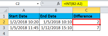
We will use the INT function to work with just the date part of the cell. This function rounds a value down to the nearest integer. So if we write the function below, this will return only the integer part of the date difference, which is the number of days.
=INT (B2-A2)
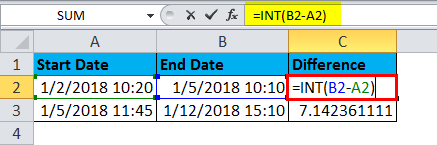
Then the result is returned as 2.
Calculating the Elapsed Hours and Minutes
We now need to work on the number of hours and minutes, which is the decimal part. We will use the MOD function to return only the decimal part of the B9-A9 formula. This function returns the remainder after a number is divided by a divisor.
We will use it to divide the B9-A9 formula by 1 so that it returns to the remainder as the decimal part. We will then use the HOUR and MINUTE functions to return the hours and minutes from this decimal value.
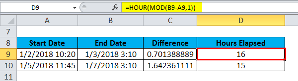
So the formula below returns the number of hours elapsed.
=HOUR(MOD(B9-A9,1))
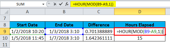
Then the result is returned as 16.
And this returns the number of minutes elapsed.
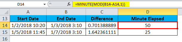
=MINUTE(MOD(B14-A14,1))
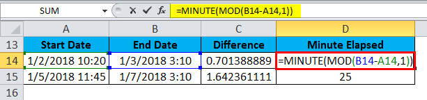
Then the result is returned as 50.
A formula for Elapsed Time in Days, Hours, and Minutes
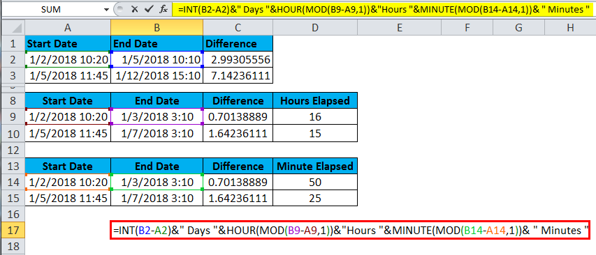
Finally, we need to put this all together as one Excel formula. We can use the ampersand (&) to concatenate the different parts of the formula. You can construct the result to look however you want. For example, the formula below would return the result as 2 days, 23 hours, and 50 minutes.
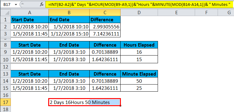
=INT(B2-A2)&” Days “&HOUR(MOD(B9-A9,1))&” Hours “&MINUTE(MOD(B14-A14,1))& ” Minutes ”
The result will return as 2 days, 16 hours, and 50 minutes.
Recommended Articles
This has been a guide to TIME in Excel. Here we discuss the TIME Formula in Excel and how to use the TIME Function in Excel, along with Excel examples and downloadable Excel templates. You may also look at these useful functions in Excel –