Updated May 29, 2023
Introduction to Compare Two Lists in Excel
Data matching or comparison in different data sets is not new in data analysis today. SQL Join method allows joining two tables having similar columns. But how do we know that there are similar columns in both tables? MS Excel allows comparing two lists or columns (Compare Two Lists in Excel) to verify if there are any common value(s) in both lists. Comparing two sets of lists may vary as per the situation. Using MS Excel, we can match two data sets and verify whether there is any common value in both sets. Excel does calculations but is useful in various ways like comparing data, data entry, analysis, visualization, etc. Below is an example that shows how data from two tables are compared in Excel. We’ll check each value from both data sets to verify common items in both lists.
How to Compare Two Lists in Excel?
Let’s understand how to compare two lists in Excel with a few examples.
Example #1 – Using the Equal Sign Operator
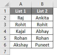
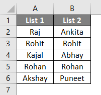
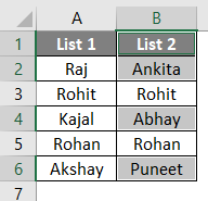
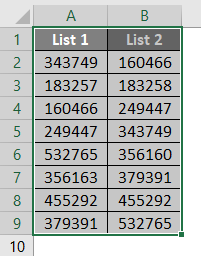
Below are two lists called List1 and List2 which we’ll compare.
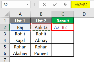
Now, we’ll insert another column called “Result” to display the result as TRUE or FALSE. If there is a match in both cells in a row, it will show TRUE; otherwise, it will show FALSE. We’ll use the Equal sign operator for the same.
After using the above formula, the output is shown below.
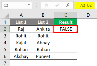
The formula is =A2=B2, which states cell A2 is compared with cell B2. A1 has “Raj”, and B1 has “Ankita”, which does not match. So, it will show FALSE in the first row of the result column. Similarly, the rest of the rows can be compared. Alternatively, we can drag the cursor from C2 to C6 to get the result automatically.
Example #2 – Match Data using the Row Difference Technique
To demonstrate this technique, we’ll use the same data as above.
First of all, the entire data is selected.
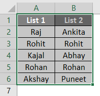
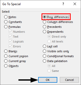
Then by pressing the F5 key on the keyboard, the “Go to special” dialog box opens. Then go to Special, as shown below.
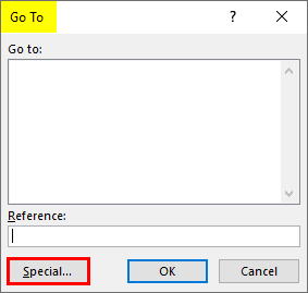
Now, select “Row difference” from the options and press OK.
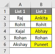
Now, matching cells are white, and unmatched cells are white and grey, as shown below.
We can highlight the row difference values for different colors at our convenience.
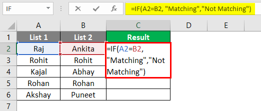
Example #3 – Row Difference using IF Condition
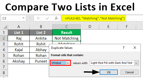
If the condition states that there is any match in the row. If there’s a match, the result will be “Matching” or “Not Matching”. The formula is shown below.
After using the above formula, the output is shown below.
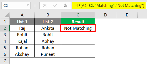
Here A2 and B2 values don’t match, so that the result will be “Not Matching”. Similarly, other rows can result with the condition, or alternatively, we can drag the cursor, and the output will come automatically as below.
Example #4 – Matching Data in Case of Row Difference
This technique is not always accurate as values may be in other cells too. So, different techniques are used for the same.
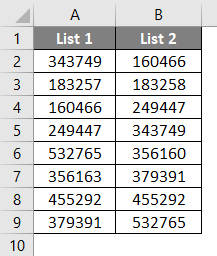
Now we’ll apply the V-Lookup function to get the result in a new column.
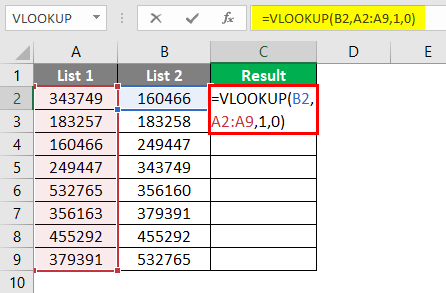
After applying the formula, the output is shown below.
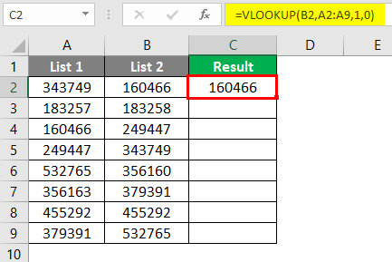
Here, the function states that B2 is being compared with values from List 1. So, the range is A2:A9. And the result can be seen as shown below.
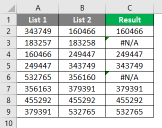
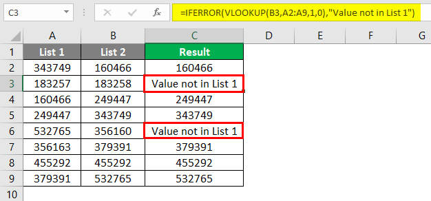
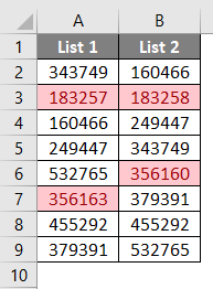
If 160466 is in any cell in List 1, then 160466 will be printed using V-Lookup. Similarly, the rest values can be checked. In the 2nd and 5th rows, there is an error. It is because values 183258 and 356160 are not present in List 1. For that, we can apply the IFERROR function as follows. Now, the result is finally here.
Example #5 – Highlighting Matching Data
Sometimes, we feel fed up with Excel formulas. So, we can use this method to highlight all the matching data. This method is conditional formatting. First, we’ll have to highlight the data.
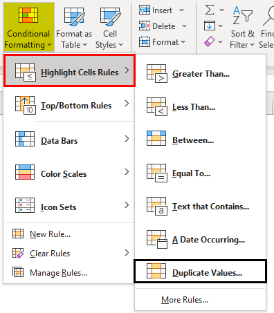
Next, we have to go to Conditional formatting > Highlight cell rules > Duplicate values, as shown below.
Then a dialog box appears as below.
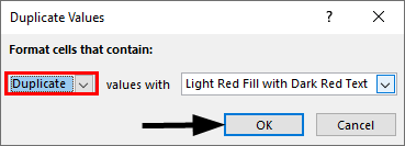
We can choose a different color from the drop-down list or stick with the default one, as shown above. Now the result can be seen below.
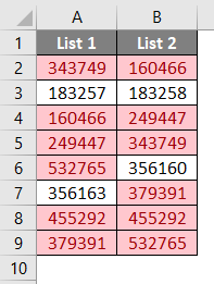
Here common values are highlighted in red color while unique values are colorless. We can color only unique values if we need to find unmatched values. For that, instead of selecting “duplicate” in the Duplicate values dialog box, we’ll select “Unique” and then press OK.
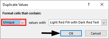
Now, the result is shown below.
Here, only unique and unmatched values are highlighted in red.
Example #6 – Partial Matching Technique
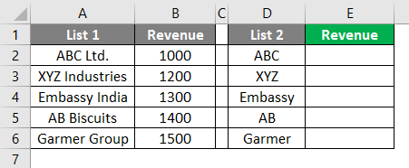
Sometimes both lists don’t have the exact data. For example, formulas or matching techniques won’t work here if we have “India is a country” in List 1 and “India” in List 2. Because List 2 has partial information about List 1. In such cases, the special character “*” can use. Below are two lists with company names with their revenue.
Here, we’ll apply V-Lookup using the special character “*” shown below.
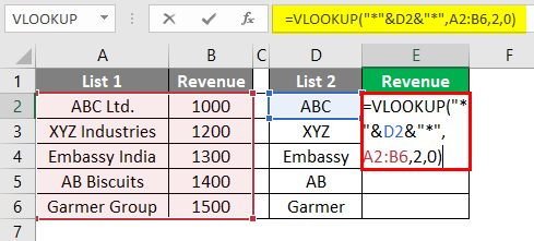
Now, we can see that 1000 is printed in cell E2. We can also drag the formula till cell E6 to the result in other cells.
Things to Remember
- The above techniques depend on the data structure of the table.
- V-Lookup is the common formula to use when the data is not organized.
- Row by row technique works in the case of organized data.
Recommended Articles
This is a guide to Compare Two Lists in Excel. We discuss How to Compare Two Lists in Excel, practical examples, and a downloadable Excel template. You can also go through our other suggested articles –
