Updated June 8, 2023

Excel Auditing Tools (Table of Contents)
Introduction to Auditing Tools in Excel
We all know why Excel is so popular throughout the world. Because of its wide range of formulae, functions, and macros, it can almost surely handle every task of the world with ease. All these formulae are easy to use, but it becomes a tough job when using multiple formulae in combination. It sometimes does not give the result as expected. It becomes easy to trace back the errors if formulae are quite simple. However, when we start creating some complex formulae, it becomes a hectic job to track the errors with such formulae. Thus, it becomes an important job for the user to be able to trace back the errors. Fortunately, Excel provides a variety of built-in tools that allow you to audit the errors with formulae and correct the same.
We have six main tools under Excel for formulae auditing listed below:
- Trace Precedents
- Trace Dependents
- Remove Arrows
- Show Formulas
- Error Checking (includes Error Checking, Trace Error, Circular References)
- Evaluate Formula
Let’s explore each of these formula auditing tools under Excel.
Examples of Auditing Tools in Excel
Lets us discuss examples of Auditing Tools in Excel.
Example #1 – Trace Precedents
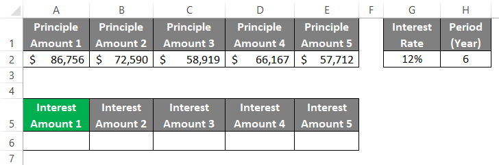
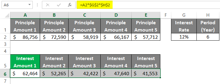
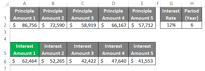
Trace precedents are the cells affecting the values/formulae under the selected cell. Suppose we have five principle amounts that we can invest with a rate of interest of 12% and a period of 6 years. We have calculated the interest amounts for all five principles using a simple formula Principle*Interest Rate*Period(in years). See the screenshot below:
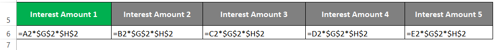
Now, if we click on cell A6 and press F2, we can see the formula we used to capture Interest Amount 1.
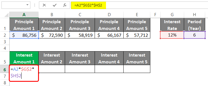
This clearly shows us that Interest Amount 1 is based on Principle Amount 1 Value (A2) and Interest Rate (H2) as well as Period (I2). However, Excel has its way of showing this relationship through cell precedents under the formula auditing group.
Step 1: Select cell A6 from the current worksheet and click on the Formulas tab at the Excel ribbon.

Step 2: Once you click on the Formulas tab, you can see the Formula Auditing group under it with various formula auditing options available.

Step 3: Click on the Trace Precedents option under the Formula Auditing group, and it will make a connection between all the cells that are affecting the currently selected cell through blue-colored arrows as shown below:
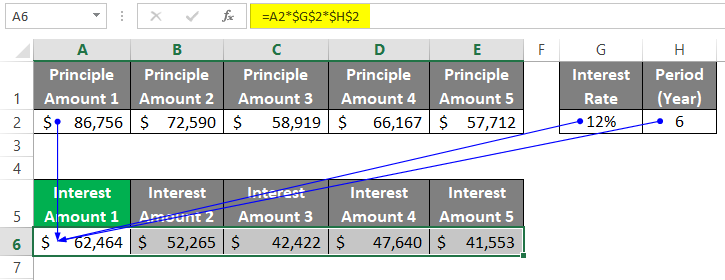
Trace Precedents help you find out what cells are associated with the formula using which the values are obtained.
Example #2 – Remove Arrows
Trace Precedents were nice since they let us see the relationship between different cells in our Excel sheet. However, we don’t want those here in our file. We wanted those to remove. Is it Possible? Well, possible!
Go again to the Formula Auditing group (Select the Formulas tab through the ribbon if you are not there and you can see this group within it). Click on the Remove Arrows dropdown.
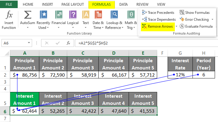
Once you click on the Remove Arrows dropdown, you can see a list of options as shown below:
You can either hit the first option, which removes all the arrows (precedents and dependents), or you can select particular options that remove the precedents or the dependents.
Example #3 – Trace Dependents
Suppose we click on any cell and want to check the cells that depend on the currently selected cell. Can we do that in Excel? Surely, we can do this. Trace Dependents is the function that shows a relationship between the selected cell and all other cells that depend on the selected cell.
Suppose we select the cell H2 (Interest Rate). And wanted to check what are all the other cells which have a dependency on H2. We can do this in Excel.
Step 1: Select cell G2 in your Excel sheet.
Step 2: Now click the Formulas tab on the Excel ribbon and select Trace Dependents to see all the cells dependent on G2.

Once you click on Trace Dependents, you’ll see all the cells that have a dependency on G2, and they will be connected with blue arrows.
Example #4 – Show Formula
See Formulas is an exciting feature within Excel that shows you the formulas under all cells (formulated) instead of the values.
Go to the Formulas tab through the Excel ribbon and click the Show Formulas button under the Formula Auditing group to see all the formulas in the current Excel sheet.

Once you click on the Show Formulas button, you can see all the formulated cells with formulas instead of values, as shown below:
Example #5 – Error Checking
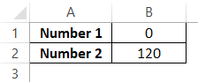
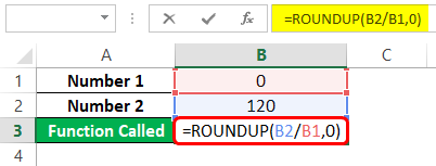
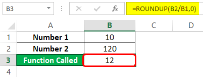
Suppose we have two numbers, Number 1 and Number 2, respectively, as shown in the image below:
Now, we call a function that takes these two cell references and should give some output. I will be using the ROUNDUP function in Excel. See cell B3 for more references.
I used the ROUNDUP function to divide 120 by zero and round it up to the nearest integer. Hit enter to see the output of this formula.
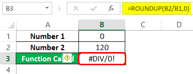
Oh, Crap! I am getting an error here. How can I check the error? Well, Excel has an Error Checking option with it.
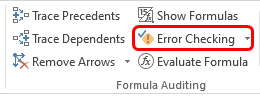
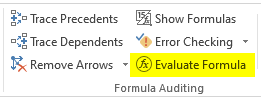
- Go to the Formula Auditing group and click on the Error Checking button.
Error Checking dialogue box will open up as shown below:
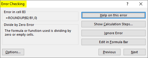
You can see online help on this error by clicking Help on this Error button, or you can see the calculation steps involved in this error by hitting Show Calculation Steps, or you can ignore the error or Edit the formula.
Click on Help on this Error button, and you’ll be redirected to Office Support online page as shown below:
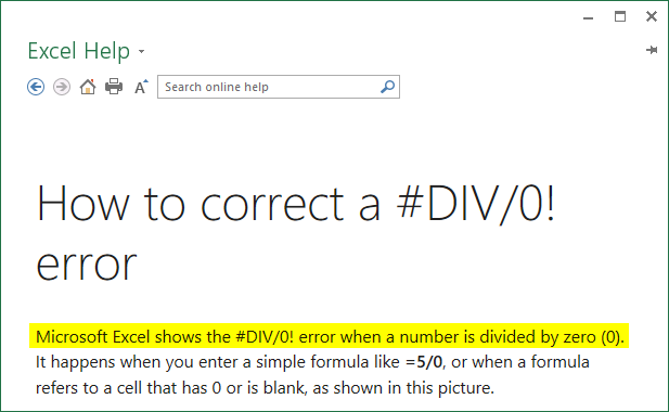
From here, I get that the #DIV/0! An error occurs when we try to divide some number with zero. I will change the value of Number 1 under cell B1 and see how the formula works in B3.
This is how error checking helps you in Excel.
Example #6 – Evaluate Formula
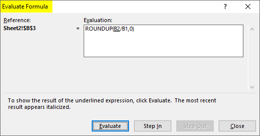
You can also evaluate any formula in Excel to see how that works. Just click on the Evaluate Formula button under the Formula Auditing group. Then you’ll see a new window where you can click the evaluate button and see the actual evaluation of the formula step by step.
This is how the Auditing Excel formula works under Excel. Now, let’s wrap things up with some points to be remembered:
Things to Remember
- The formula Auditing tool can be found under the Formula tab and has a separate group assigned to it.
- There is a keyboard shortcut for the Show Formula option. You can directly hit “Ctrl + `” simultaneously from your keyboard to Show Formulas in the entire sheet.
- You can also use the F9 button to Evaluate the Formula within that option.
Recommended Articles
This has been a guide to Auditing Tools in Excel. Here we discuss How to use Auditing Tools in Excel, practical examples, and a downloadable Excel template. You can also go through our other suggested articles –
