Updated May 29, 2023
What If Analysis In Excel (Table of Contents)
Overview of What If Analysis in Excel
What-if analysis in Excel tests more than one value for a different formula based on multiple scenarios. For this, we must have data of such kind where, for a single parameter, we would have 2 or more values for comparison. Go to the Data menu tab and click the What-If Analysis option under the Forecast section. Select the scenario manager, give a scenario name, and select the scenario value cell. Now from the Goal Seek option from What-If Analysis, determine the value we want to compare. By this, we can enter multiple scenarios.
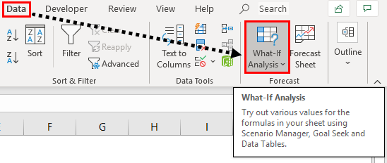
What if the analysis is available in the “forecast” section under the “Data” tab.
There are three different kinds of tolls in the What-if analysis. Those are:
1. Scenario manager
2. Goal Seek
3. Data table
We will see each one with related examples.
Examples of What If Analysis in Excel
Here are some examples given below:
Example #1 – Scenario Manager
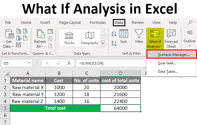
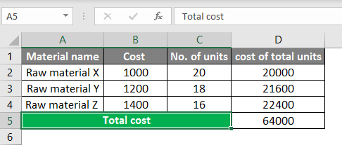
The scenario manager helps to find the results for different scenarios. Let’s consider a company that wants to buy raw materials for their organization’s needs. Due to the scarcity of funds, the company wants to understand how much cost will happen for different possibilities of buying.
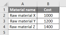
In these cases, we can use the scenario manager to apply different scenarios to understand the results and make the decision accordingly. Now consider Raw Material X, Raw Material Y, and Raw Material Z. We know the price of each, and we want to know how much amount needed for different scenarios.
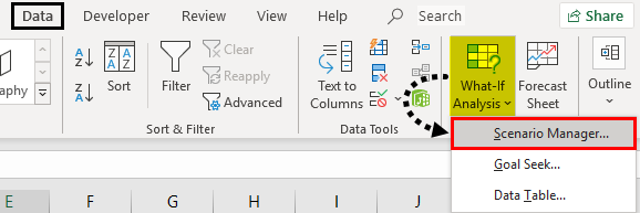
Now we need to design 3 scenarios like High volume purchase, Medium volume purchase, and Low volume purchase. For that, click on What if Analysis and select Scenario Manager.
Once we select the scenario manager, the following window will open.
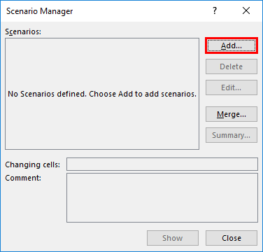
As shown in the screenshot, currently, there are no scenarios; if we want to add scenarios, we need to click on the “Add” option available.
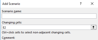
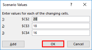
Then it will ask for the Scenario name and changing cells. Give a scenario name whatever you want as per your requirement. Here I am giving “High volume.”
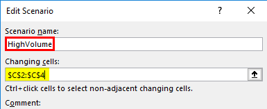
Changing cells is the range of cells your scenario values for different scenarios. Suppose we observe the below screenshot. No. of units will change in each scenario; that is the reason for changing cells; we used C2:C4, which means C2, C3, and C4.
Once you give the change values, click on “OK”, then it will ask for the changing values for the High volume scenario. Input the values for the high volume scenario and then click “Add” to add another scenario “, Medium Volume.”
Give the name “Medium volume,” give the same range and click Ok, then it will ask for values.
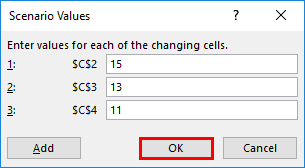
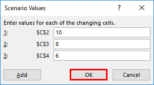
Again, click “Add” and create one more scenario “, Low volume”, with low values like the one below.
Once all scenarios have been done, click on “Ok” You will find the below screen.
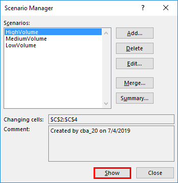
We can find all the scenarios on the “Scenarios” screen. Now we can click on each scenario and Show; then, you will find the results in Excel; otherwise, we can view all the scenarios by clicking on the option “Summary.”
If we click on the scenario wise, the results will be changed in Excel as below.
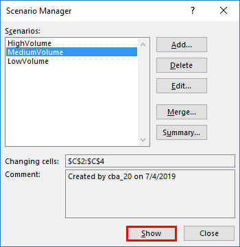
Whenever you click on the scenario and show the results at the back will change. If we want to see all the scenarios at a time to compare with others, click on the summary the following screen will come.
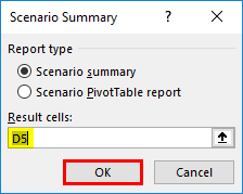
Select ‘Scenario Summary” and give the “Results Cells” here; the total results will be in D5; hence I given D5, click ‘Ok’. Then a new tab will be created named “Scenario summary.”
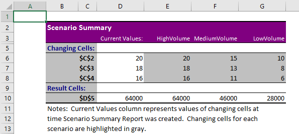
Here the columns in grey are the changing values, and the column in white is the current value which was the last selected scenario results.
Example #2 – Goal Seek
Goal seek helps to find the input for the known output or required output.
Suppose we will take a small example of a product sale. Suppose we know that we want to sell the product at an additional price of 200 than the product cost. Then we want to know what percentage we are earning the profit.
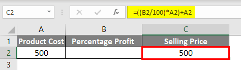
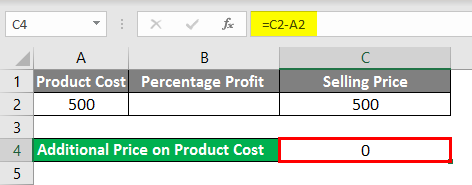
Observe the above screenshot product cost is 500, and I have given the formula for finding the percentage profit, which you can observe in the formula bar. In one more cell, I gave the formula for the additional price we want to sell.
Now use Goal Seek to find the profit percentage of the different additional prices on the product’s cost and selling price.
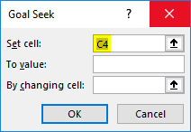
When we click “Goal seek”, the above pop up will come. In the set, the cell gives the cell position where we will give the output value here, the additional price amount we know, which we give in cell C4.
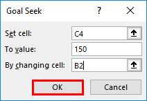
The “To Value” is the value at what additional price we want to cell 150 rupees additional to the product cost, and the changing cell is B2 where percentage changes. Click on “Ok” and see how much the percentage profit is if we sell an additional 150 rupees.
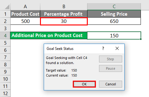
The profit percentage is 30, and the selling price should be 650. Similarly, we can check for different targeted values. This goal seeks to help to find the EMI calculations etc.
Example #3 – Data Tables in What If Analysis
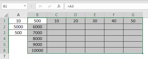
Now we will see the Data table. We will consider a very small example to understand better. Suppose we want to know the 10%, 20%, 30%, 40%, and 50% of 5000; similarly, we want to find the percentages for 6000, 7000, 8000, 9000, and 10000.
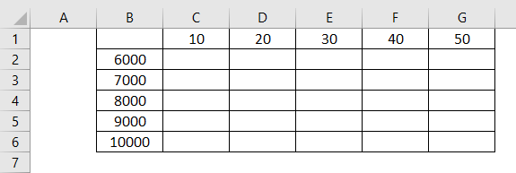
We have to get the percentages in each combination. In these situations, the Data table will help to find the output for a different combination of inputs. Here in Cell B3 should get 10% of 6000 and B4 10% of 7000 and so on. Now we will see how to achieve this. First, create a formula to perform this.
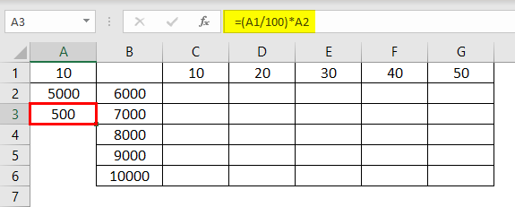
If we observe the above screenshot, the part marked with a box is the example. In A3, we have the formula to find the percentage from A1 and A2. So inputs are A1 and A2. Now take the result of A3 to A1, as shown in the below screenshot.
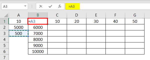
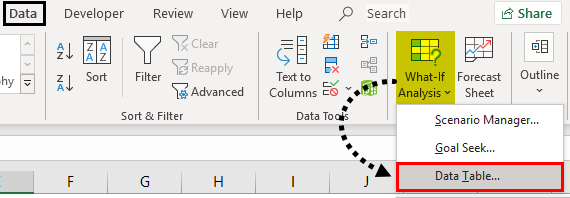
Now select the entire table to apply the Data table of What if Analysis shown in the screenshot below.
Once selected, click on “Data” and then “What If Analysis” from that dropdown, select data table.
Once you select “Data table”, the below pop-up will come.
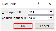
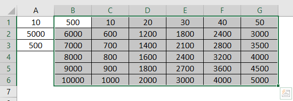
In “Row Input cell”, give the cell address where the row inputs should be input, which means here, row inputs are 10, 20, 30,40, and 50. Similarly, give “Column input cell” as A2 here. Column inputs are 6000, 7000, 8000, 9000, and 10,000. Click on “Ok”, then results will appear as a table, as shown below.
Things to Remember
- What if Analysis is available under the “Data” menu on the top.
- It will have 3 features 1. Scenario manager 2. Goal seeks, and 3. Data table.
- Scenario manager helps to analyze different situations.
- Goal seeking to know the right input value for the required output.
- The data table helps to get results of different inputs row-wise and column-wise.
Recommended Articles
This is a guide on What if Analysis in Excel. Here we discuss three tools in What If Analysis and the examples and downloadable Excel template. You may also look at the following articles to learn more –
