Updated July 3, 2023
What are Sparklines in Excel?
Sparklines are small, simple charts designed to fit in a single cell and show trends and variations in data. They provide a quick visual representation of data that is easy to read and understand. Sparklines in Excel can help track sales figures, and website traffic, monitor stock prices and currency exchange rates, or track student performance over time.
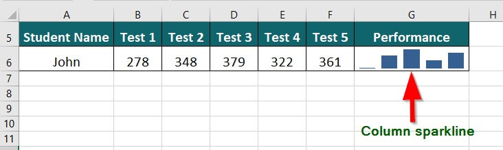
For instance, you can use a Column sparkline to visualize a student’s performance in various tests, as shown in the image below.
Types of Sparklines in Excel
Excel offers three types of sparklines that help users represent data: Line, Column, and Win/Loss sparklines.
- Line: This type of sparkline represents the data trend over time using a continuous line. It does not display magnitude or axes. It helps show patterns and trends in data.

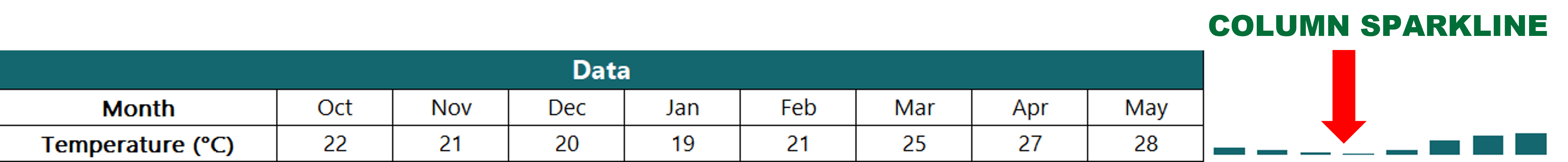
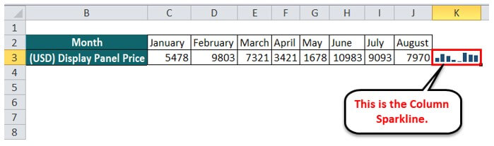
- Column: This type of sparkline shows the data trend using vertical columns. Column sparklines help compare data values and identify low and high points.
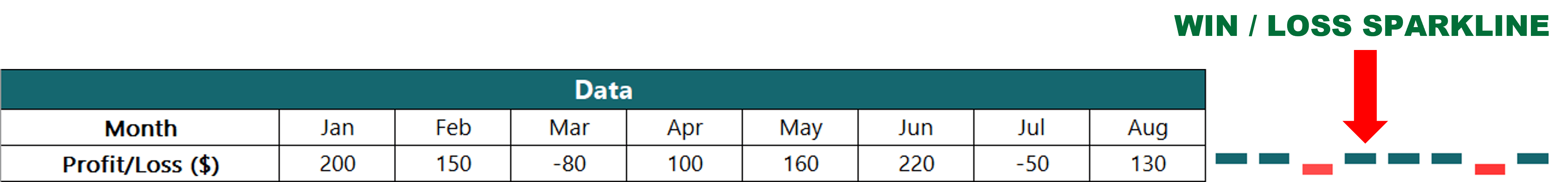
- Win/Loss: It displays the data trend as positive or negative symbols. Win/ Loss sparklines help display changes in data values that represent gains or losses.
How to Create a Sparklines in Excel?
To create Sparklines in Excel, follow the below-given steps:
- Select the desired cell to insert the sparkline.
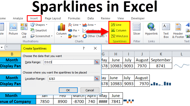
- Click on the Insert tab on the Excel ribbon.
- In the Sparklines group, choose the desired sparkline type (Line, Column, or Win/ Loss).
- In the Data Range field of the Create Sparklines window, select the cell range containing the data you want to display in the Sparkline.
- In the Location Range field, select the cell where you want to insert the sparkline.
- Click
To understand the above steps better, let’s explore some examples:
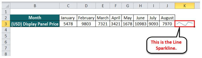
Example #1 Data Representation Using Line Sparkline
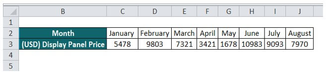
The following example shows the fluctuating prices of Display Panel across various months. We want to represent the same using the Sparkline feature of Excel.
Solution:
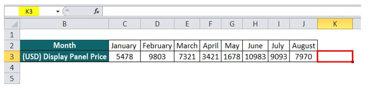
Step 1: Select an empty cell (Cell K3) where you want to insert the sparkline.
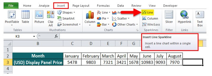
Step 2: Navigate to the Insert tab and select the Line option from the Sparklines menu.
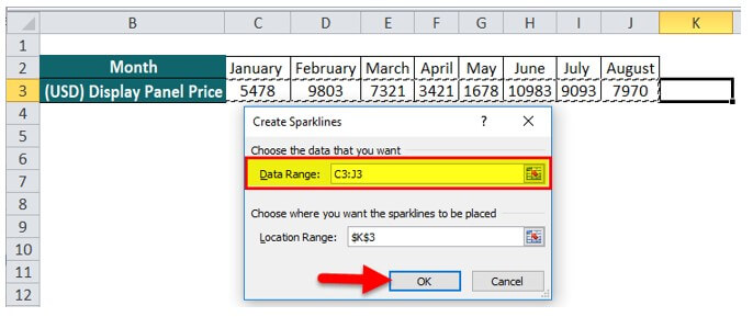
A Create Sparklines dialog box appears on the screen.
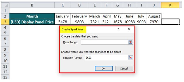
Step 3: Select the appropriate data range( C3:J3) in the designated Data Range box. Since we have already selected the desired cell (K3) to display the sparkline, the Location Range box is automatically populated.
Step 4: Click OK to insert the sparkline.
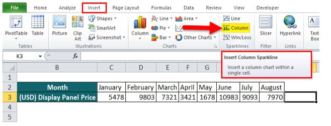
Example #2 Data Representation Using Column Sparkline
Consider the same example of fluctuating Panel prices, which we want to represent using column sparklines.
Solution:
Step 1: Select an empty cell (Cell K3) where you want to insert the sparkline.
Step 2: Go to Insert and choose Column from the Sparklines menu.
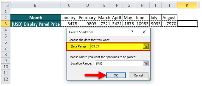
Step 3: In the Create Sparklines window, specify the data range (C3:J3), and the Location Range is automatically filled with the desired cell (K3), as you have already selected it.
Step 4: Press OK.
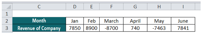
Example #3 Data Representation Using Win/ Loss Sparkline
The following example illustrates a company’s revenue performance over six months, and we want to visualize the same in terms of profit or loss using Win/ Loss sparkline in Excel.
Solution:
Step 1: Select an empty cell (Cell J3) where you want to insert the Sparkline.
Step 2: Go to Insert and choose Win/Loss from the Sparklines menu.
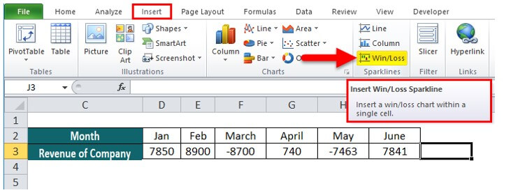
A Create Sparklines dialog box will appear.
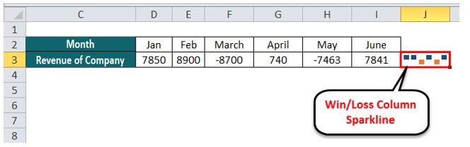
Step 3: Select the data range as D3:I3 and the location range as J3.
Step 4: Click OK.

How to Update Sparklines in Excel?
Sometimes you require adding or removing entries from an existing dataset and would like the changes to reflect in the Sparkline visualization.
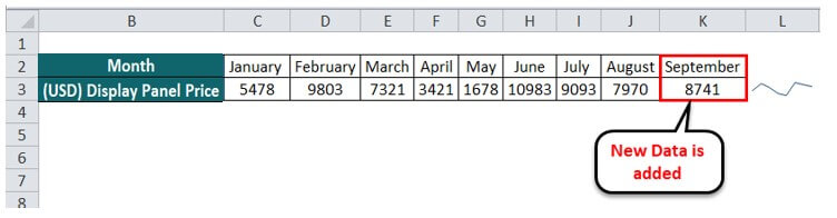
Consider the example where we add a Display Panel Price for September and want to display the corresponding changes in the Sparkline.
Solution:
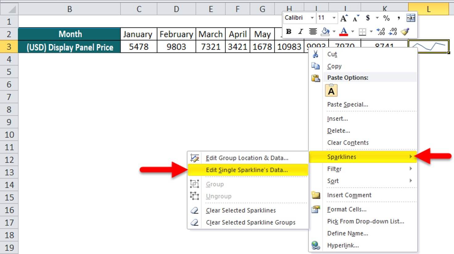
Step 1: Right-click on the cell containing Sparkline.
Step 2: In the context menu, go to Sparklines, and click Edit Single Sparkline’s Data.
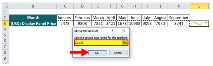
An Edit Sparkline Data dialog box appears.
Since we have added new data, we need to update the data range in the dialog box.
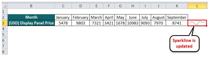
Step 3: Specify the new data range (C3:K3) and click OK.
Advantages of Sparklines
- Easy to Read: Sparklines are small in size, which makes them easy to read and helpful for quickly identifying trends and patterns in data.
- Space-saving: Sparklines take up less space than traditional charts due to their small and compact size. This feature may be helpful when a user wants to visualize multiple data sets on a single worksheet.
- Contextual visualization: Sparklines may provide valuable insights/ contexts, enabling users to see patterns and trends in data at a glance. It can be helpful to make more informed decisions and identify critical areas requiring further analysis.
- Compatibility: Sparklines are entirely integrated with Excel, enabling users to use it alongside other Excel features.
Disadvantages of Sparklines
- Limited customization: The sparkline feature of Excel provides limited customization options compared to other charts, which can be a drawback when a user wants to create a more complex visualization.
- Lack of context: Excel’s Sparklines feature does not provide enough details, such as the lack of axes and labels. Due to this, a new user might find it difficult to interpret data accurately.
- Limited data range: Excel’s Sparkline can work with only small data sets and become less effective as the data range grows. Therefore, we cannot use it to visualize complex datasets.
Things to Remember
- Excel updates the Sparklines automatically when there is a change in the source data. However, if the data range is modified or altered, it won’t reflect in the sparkline visualization.
- You can resize the sparkline by adjusting the cell’s height or width. It can help you customize the size and layout of your sparklines to fit your specific needs.
- Select a single row or column when specifying the Location Range for your sparklines. If you select multiple rows or columns, it may result in an error. For example, if you choose two rows instead of one, Excel may prompt you to “Select a single row or column”.
- Sparklines can represent hidden or empty cells, allowing you to visualize trends even if data is missing. Suppose you have a sales data table, but some cells are empty because there are no sales during a particular period. In this case, you can use a win-loss sparkline to easily visualize sales trends over time, even if some values are missing in your data set.
Frequently Asked Questions (FAQs)
Q1. How do I show Sparklines in Google Sheets?
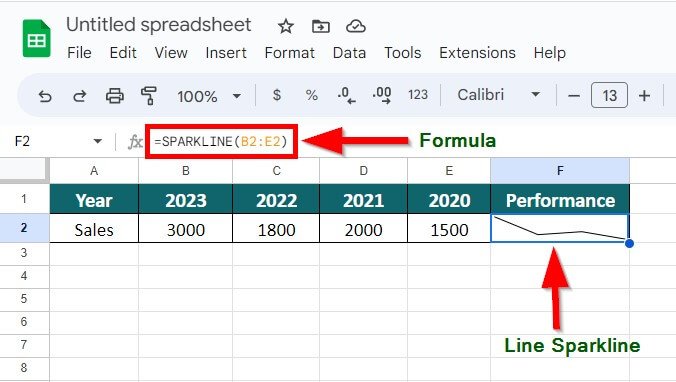
Answer: To show sparklines in Google Sheets, insert the formula =SPARKLINE(range) and press Enter. The formula will insert a line sparkline by default, as illustrated in the image below.
Q2. How do I add multiple sparklines in Excel?
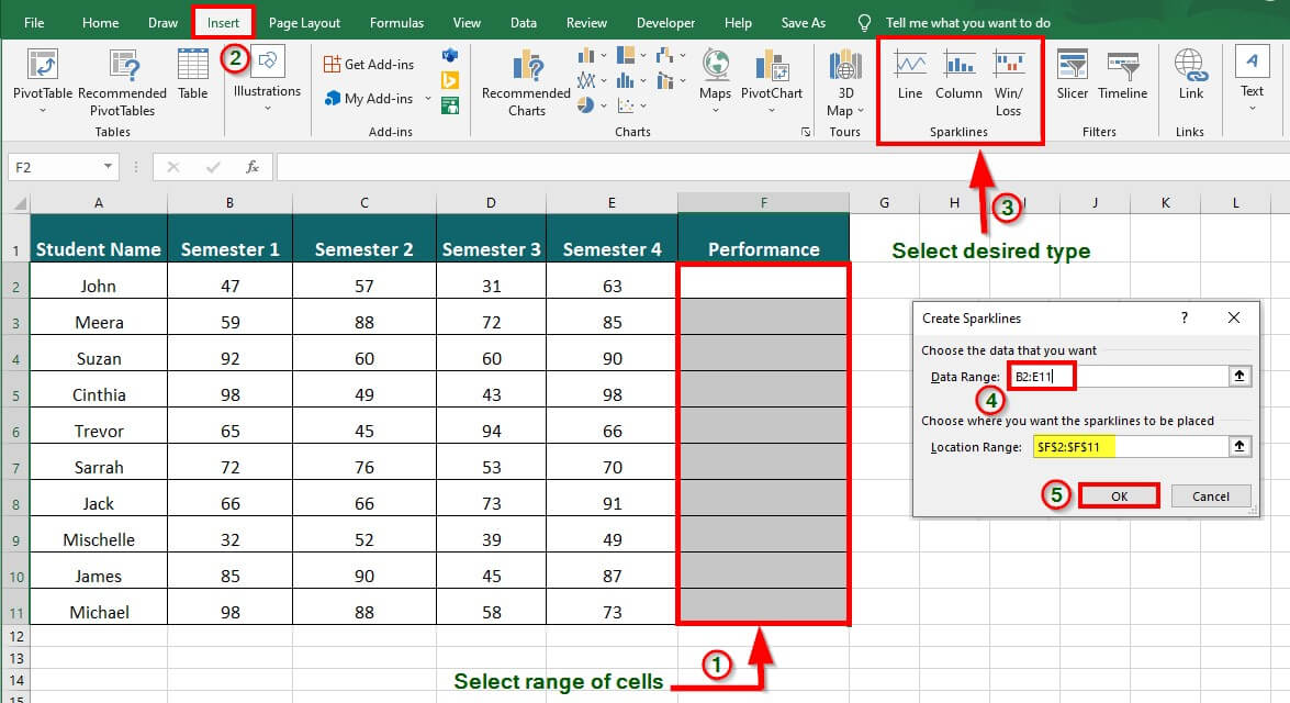
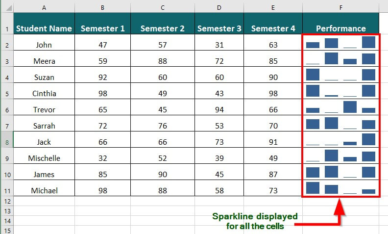
Answer: To insert Sparklines to multiple cells, follow these steps:
Step 1: Select the cell range where you want to display the graph
Step 2: Go to Insert and choose the desired Sparline type.
Step 3: In the Create Sparklines dialog box, select all the data for which you want to create a sparkline( B2:E11)
(The Location Range is auto-filled since we had already selected the cell range for displaying the output).
Step 4: Click OK.
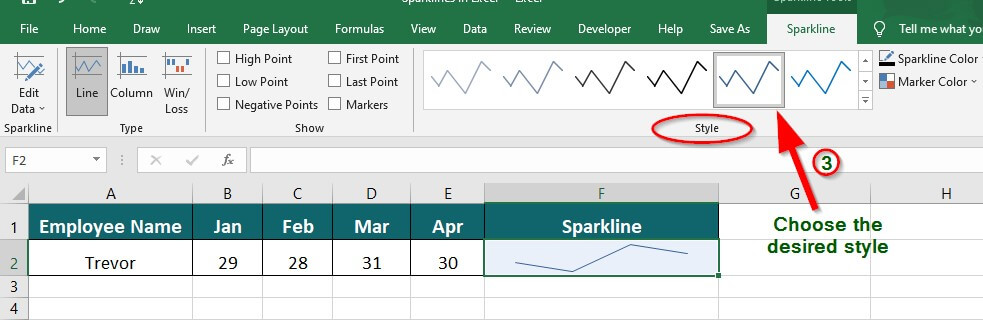
Q3. Where are sparkline styles in Excel?
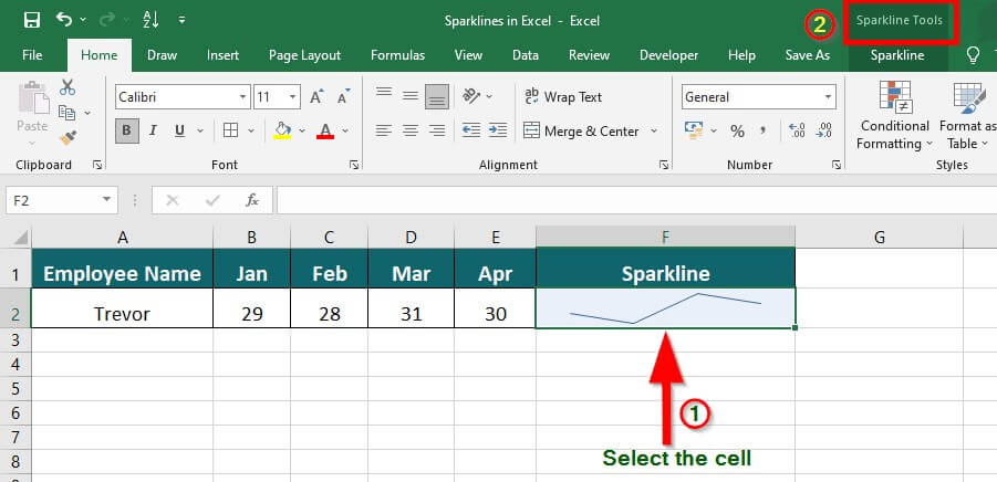
Answer: To locate sparkline styles in Excel, follow these steps:
Step 1: Select the cell containing the sparkline
Step 2: Go to Sparkline Tools
Step 3: Choose the desired Sparkline style from the Style group.
Q4. Can you conditional format sparklines?
Answer: You cannot edit conditional format sparklines in Excel.
Recommended Articles
It has been a guide to Sparklines in Excel. Here we discuss its types, how to create Sparklines in Excel, Excel examples, and a downloadable Excel template. You may also look at these suggested articles to learn more –
