Updated April 6, 2023
Introduction to Single Layer Perceptron
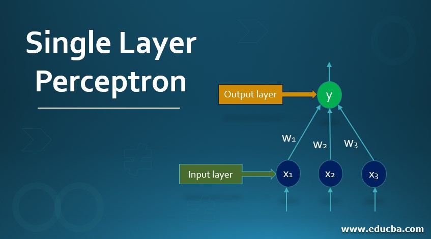
In this article we will go through a single-layer perceptron this is the first and basic model of the artificial neural networks. It is also called the feed-forward neural network. The working of the single-layer perceptron (SLP) is based on the threshold transfer between the nodes. This is the simplest form of ANN and it is generally used in the linearly based cases for the machine learning problems.
Working of Single Layer Perceptron
The SLP looks like the below:
Let’s understand the algorithms behind the working of Single Layer Perceptron:
- In a single layer perceptron, the weights to each input node are assigned randomly since there is no a priori knowledge associated with the nodes.
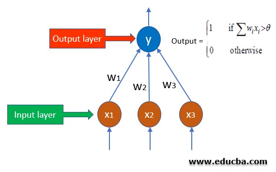
- Also, a threshold value is assigned randomly
- Now SLP sums all the weights which are inputted and if the sums are is above the threshold then the network is activated.
- If the calculated value is matched with the desired value, then the model is successful
- If it is not, then since there is no back-propagation technique involved in this the error needs to be calculated using the below formula and the weights need to be adjusted again.
Perceptron Weight Adjustment
Below is the equation in Perceptron weight adjustment:
Where,
- d: Predicted Output – Desired Output
- η: Learning Rate, Usually Less than 1.
- x: Input Data.
Since this network model works with the linear classification and if the data is not linearly separable, then this model will not show the proper results.
Example to Implement Single Layer Perceptron
Let’s understand the working of SLP with a coding example:
We will solve the problem of the XOR logic gate using the Single Layer Perceptron. In the below code we are not using any machine learning or deep learning libraries we are simply using python code to create the neural network for the prediction.
Let’s first see the logic of the XOR logic gate:
- 1 1 —> 0
- 1 0 —> 1
- 0 1 —> 1
- 0 0 —> 0
XOR is the Reverse of OR Gate so:
- If Both the inputs are True then output is false
- If Both the inputs are false then output is True.
- If Any One of the inputs is true, then output is true.
So, let’s get started with the coding
- We are using the two libraries for the import that is the NumPy module for the linear algebra calculation and matplotlib library for the plotting the graph.
import numpy as np
import matplotlib.pyplot as plt- Defining the inputs that are the input variables to the neural network
X = np.array([[1,1,0],[1,0,1],[1,0,0],[1,1,1]])- Similarly, we will create the output layer of the neural network with the below code
y = np.array([[1],[1],[0],[0]])- Now we will right the activation function which is the sigmoid function for the network
def sigmoid(x):
return 1/(1 + np.exp(-x))- The function basically returns the exponential of the negative of the inputted value
- Now we will write the function to calculate the derivative of the sigmoid function for the backpropagation of the network
def sigmoid_deriv(x):
return sigmoid(x)*(1-sigmoid(x))- This function will return the derivative of sigmoid which was calculated by the previous function
- Function for the feed-forward network which will also handle the biases
def forward(x,w1,w2,predict=False):
  a1 = np.matmul(x,w1)
  z1 = sigmoid(a1)
  bias = np.ones((len(z1),1))
  z1 = np.concatenate((bias,z1),axis=1)
  a2 = np.matmul(z1,w2)
  z2 = sigmoid(a2)
  if predict:
    return z2
return a1,z1,a2,z2- Now we will write the function for the backpropagation where the sigmoid derivative is also multiplied so that if the expected output is not matched with the desired output then the network can learn in the techniques of backpropagation
def backprop(a2,z0,z1,z2,y):
  delta2 = z2 - y
  Delta2 = np.matmul(z1.T,delta2)
  delta1 = (delta2.dot(w2[1:,:].T))*sigmoid_deriv(a1)
  Delta1 = np.matmul(z0.T,delta1)
return delta2,Delta1,Delta2- Now we will initialize the weights in LSP the weights are randomly assigned so we will do the same by using the random function
w1 = np.random.randn(3,5)
w2 = np.random.randn(6,1)- Now we will initialize the learning rate for our algorithm this is also just an arbitrary number between 0 and 1
lr = 0.89
costs = []- Once the learning rate is finalized then we will train our model using the below code.
epochs = 15000
m = len(X)
for i in range(epochs):
a1,z1,a2,z2 = forward(X,w1,w2)
delta2,Delta1,Delta2 = backprop(a2,X,z1,z2,y)
w1 -= lr*(1/m)*Delta1
w2 -= lr*(1/m)*Delta2
c = np.mean(np.abs(delta2))
costs.append(c)
if i % 1000 == 0:
print(f"iteration: {i}. Error: {c}")
print("Training complete")- Once the model is trained then we will plot the graph to see the error rate and the loss in the learning rate of the algorithm
z3 = forward(X,w1,w2,True)
print("Precentages: ")
print(z3)
print("Predictions: ")
print(np.round(z3))
plt.plot(costs)
plt.show()
Example
The above lines of code depicted are shown below in the form of a single program:
import numpy as np
import matplotlib.pyplot as plt
#nneural network for solving xor problem
#the xor logic gate is
# 1 1 ---> 0
# 1 0 ---> 1
# 0 1 ---> 1
# 0 0 ---> 0
#Activation funtion
def sigmoid(x):
    return 1/(1 + np.exp(-x))
#sigmoid derivative for backpropogation
def sigmoid_deriv(x):
    return sigmoid(x)*(1-sigmoid(x))
#the forward funtion
def forward(x,w1,w2,predict=False):
    a1 = np.matmul(x,w1)
z1 = sigmoid(a1)
#create and add bais
bias = np.ones((len(z1),1))
z1 = np.concatenate((bias,z1),axis=1)
a2 = np.matmul(z1,w2)
z2 = sigmoid(a2)
if predict:
    return z2
return a1,z1,a2,z2
def backprop(a2,z0,z1,z2,y):
    delta2 = z2 - y
Delta2 = np.matmul(z1.T,delta2)
delta1 = (delta2.dot(w2[1:,:].T))*sigmoid_deriv(a1)
Delta1 = np.matmul(z0.T,delta1)
return delta2,Delta1,Delta2
#first column = bais
X = np.array([[1,1,0],
[1,0,1],
[1,0,0],
[1,1,1]])
#Output
y = np.array([[1],[1],[0],[0]])
#initialize weights
w1 = np.random.randn(3,5)
w2 = np.random.randn(6,1)
#initialize learning rate
lr = 0.89
costs = []
#initiate epochs
epochs = 15000
m = len(X)
#start training
for i in range(epochs):
    #forward
    a1,z1,a2,z2 = forward(X,w1,w2)
#backprop
delta2,Delta1,Delta2 = backprop(a2,X,z1,z2,y)
w1 -= lr*(1/m)*Delta1
w2 -= lr*(1/m)*Delta2
# add costs to list for plotting
c = np.mean(np.abs(delta2))
costs.append(c)
if i % 1000 == 0:
    print(f"iteration: {i}. Error: {c}")
#training complete
print("Training complete")
#Make prediction
z3 = forward(X,w1,w2,True)
print("Precentages: ")
print(z3)
print("Predictions: ")
print(np.round(z3))
plt.plot(costs)
plt.show()
Output:
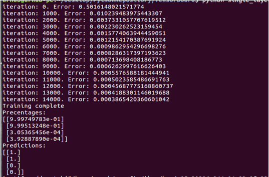
Explanation to the above code: We can see here the error rate is decreasing gradually it started with 0.5 in the 1st iteration and it gradually reduced to 0.00 till it came to the 15000 iterations. Since we have already defined the number of iterations to 15000 it went up to that.
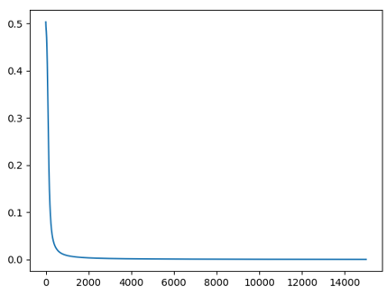
Graph Explanation
We can see the below graph depicting the fall in the error rate
Advantages and Disadvantages
Below we discuss the advantages and disadvantages for the same:
Advantages
- Single-Layer Perceptron is quite easy to set up and train.
- The neural network model can be explicitly linked to statistical models which means the model can be used to share covariance Gaussian density function.
- The SLP outputs a function which is a sigmoid and that sigmoid function can easily be linked to posterior probabilities.
- We can interpret and input the output as well since the outputs are the weighted sum of inputs.
Disadvantages
- This neural network can represent only a limited set of functions.
- The decision boundaries that are the threshold boundaries are only allowed to be hyperplanes.
- This model only works for the linearly separable data.
Conclusion – Single Layer Perceptron
In this article, we have seen what exactly the Single Layer Perceptron is and the working of it. Through the graphical format as well as through an image classification code. We have also checked out the advantages and disadvantages of this perception.
Recommended Articles
We hope that this EDUCBA information on “Single Layer Perceptron” was beneficial to you. You can view EDUCBA’s recommended articles for more information.
