Updated March 27, 2023
Introduction to Covariance in Matlab
Covariance is one of the important parameters in the field of Statistics and Analytics. If there are two variables in a dataset, then covariance tells us how do those variables vary. It is a measure that tells us how one variable can change by changing another variable. Variance is different than covariance because variance tells us how a single variable in a dataset varies. In the field of analytics, it is used in many fields such as, it used to determine the linear relationship between the variables based on their dependency and it also gives the direction of the relationship between the variables in the dataset.
Working of Covariance in Matlab
In Matlab, there are many functions that are used for implementing the tasks in the analytics and statistics domain. Covariance is one of the important function which is used to determine the relationship between the variables. Please find the below syntaxes which are used in Matlab to determine covariance:
1. co=cov(x)
This returns the covariance of the various observations mentioned in variable x and co returns the covariance which is scalar in nature if x is a vector. If x is a matrix, then the rows of the matrix represent the random variables while the rows in them represent the different observations and the resultant co returns the covariance matrix with rows and columns where the variance is there in the diagonal. The resultant can also be normalized by the number of observations subtracted 1. If there is only one observation, then the result is normalized by 1. If the input x is scalar is nature then the covariance of it is 0, while if it is an empty array then the covariance of it is NaN.
2. co=cov (x, y)
This returns the covariance between the random variables x and y. The inputs can be of different natures like if the inputs are in the form of the matrix then the covariance treats x and y as vectors, where x and y should be of the same size. If the inputs are in the form of the vector which is of equal length, then it returns a 2 by 2 covariance matrix. If the inputs are scalar in nature then the covariance of it is 0, while if it is an empty array it returns NaN.
3. co=cov (____, weight)
This is used to specify the normalization weight for any of the syntaxes mentioned above. The value of normalization weight is 0 by default and the resultant covariance is normalized by the given number of observations subtracted by 1. If the value of normalization weight is 1, then covariance is normalized by a given number of observations.
4. co=cov (___, nanflag)
This is used to remove all NaN values which will be present by executing the above syntaxes.
- The input and output arguments in the above syntaxes should follow certain conditions and criteria which should be taken care of. The first input array x can be in the form of vector or matrix and the data types that are handled by it are single and double. Similarly, y is the second input which also can be in the form of vector or matrix; provided that the first and second input should of the same size. The data types accepted by the second input are single and double. Weight is another input argument as mentioned in the third syntax and it can take values of 0 and1.
- The data types that are accepted by weight are single and double. nanflag is another input argument which is mentioned in the fourth syntax and it can take three values as one of the input. If the value of nanflag is “includenan” then it will include all NaN values present in the input arguments before calculating the covariance. If the value of nanflag is “omitrows” then it will omit all the rows that contain NaN values before calculating the covariance. Similarly, if the value of nanflag is “partialrows” then it will remove NaN on a pairwise basis before calculating the covariance. The data type that is accepted by this is only char.
- The output argument “co” as mentioned in the above syntaxes can be in the form of scalar or matrix. If there is a single matrix input, then the output has a size similar to the number of variables present in the input argument and the variances of the columns are represented in the diagonal. If the inputs are in the form of two by two matrix, then the output argument is in the form of 2 by 2 covariance matrix representing the variance between two variables. Please find the below examples that show the use of covariance in Matlab:
Examples of Covariance in Matlab
Below are the examples of covariance in Matlab:
Example #1
To calculate the covariance of a 3 by 4 matrix:
Code:
x = [4 0 2 6; 1 -4 6 2; 3 8 7 9];

co = cov(x)
Output:
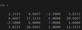
In the above example, the output shows the covariance matrix of a 3 by 4 matrix as input to it. The number of columns of the input x is 4, so the result is a 4 by 4 covariance matrix.
Example #2
To compute 2 by 2 covariance matrix by creating two matrices which are of the same size:
Code:
x = [1 0 -8; 2 3 1];

y = [4 2 5; -3 3 8];

co = cov(x,y)
Output:
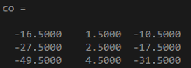
Example #3
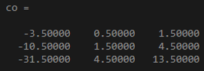
To create a matrix and calculate the covariance by normalizing the number of rows:
Code:
x = [2 4 -2; 3 8 1; -4 5 6];

co = cov(x,1)
Output:
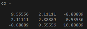
Example #4
To compute covariance of the matrix:
Code:
x = [4 3 -3; 7 8 6];

y = [9 7 10; -2 8 3];

co = cov(x,y)
Output:
Conclusion
Covariance values can lie from –infinity to +infinity; where the negative result represents a negative relationship and positive result represents a positive relationship. Covariance plays an important role in the analytics, so it is essential to know the applications of it if we are working with the related tasks.
Recommended Articles
This is a guide to Covariance in Matlab. Here we discuss the introduction, working, and examples of covariance in Matlab with proper codes and outputs. You can also go through our other related articles to learn more –
