Updated March 23, 2023
Introduction to R Normal Distribution
The following article provides an outline for R Normal Distribution. Normal Distribution is one of the fundamental concepts in Statistics. It is defined by the equation of probability density function. The probability density function is defined as the normal distribution with mean and standard deviation.
The above definition is suited in statistics, but in R, “It is the collection of data from different independent sources.” The variables are assigned on the horizontal axis, and the count of those values is on the vertical axis. The center of the curve represents the mean. In the ideal normally distributed graph, half of the variable values lie to the left, half of them to the right of the mean.
Plotting the Graph
Before we plot a graph, We need to generate a sequence of values to plot them.
In R, we use a function called seq() to generate a set of random values between two integers. Let’s generate random values that help us in plotting the normally distributed graph.
Code:
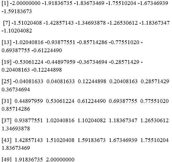
seq(-2,2,length=50)
In the above function, we generate 50 values that are in between -2 and 2. Below are the values generated and stored in the variable x.
Output:
Functions in R Normal Distribution
There are four different functions to generate a normal distribution plot.
- dnorm
- pnorm
- qnorm
- rnorm
Parameters:
- x is a vector of numbers.
- p is a set of probabilities.
- n is no. of observations.
- Mean is the mean value of the data. The default value is zero.
- sd is the standard deviation. The default value is 1.
1. dnorm()
The function is used to give the probability distribution of a specified mean and the standard deviation.
Syntax: dnorm(x, mean, sd)
x – vector of numbers. Mean-mean value of the data. The default value is zero. sd-standard deviation. The default value is 1.
Code:
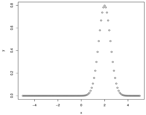
# Create a sequence of numbers between -5 and 5 incrementing it by 0.2.

x <- seq(-5, 5, by = .1)

# The mean here is 2.0 and standard deviation as 0.5.

y <- dnorm(x, mean = 2.0, sd = 0.5)

#Plot the Graph

plot(x,y)

# Saving the file.

dev.off()
Output:
Steps Used to Plot the Normal Distribution Plot:
- We have created the sequence by incrementing it by x number.
- We use the function with the standard set of parameters like mean and standard deviation.
- Plot the graph with x,y values.
- You can create the chart and save the file using the below commands.
To Give the Filename: png(file = “disnorm.png”)
To Save the File: dev.off()
2. pnorm()
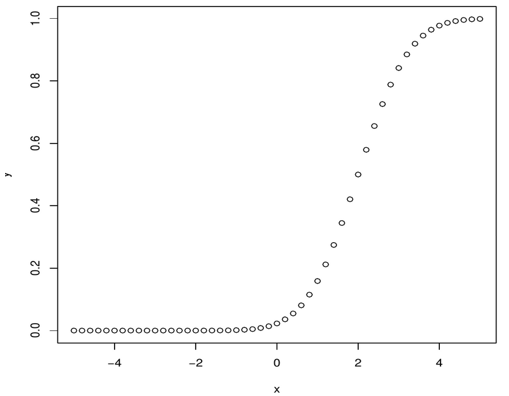
pnorm function is used to generate the cumulative distribution function. The cumulative distribution function of a random variable X, it is the probability of the value x can take that is less or equal to X.
Syntax: pnorm(x, mean, sd)
Code:
# Create a sequence of numbers between -5 and 5 incrementing by 0.2.

x <- seq(-5,5,by = .2)

# mean is 2.0 and standard deviation as 1.

y <- pnorm(x, mean = 2.0, sd = 1)

# Plot the graph.

plot(x,y)

# Saving the file.

dev.off()
Output:
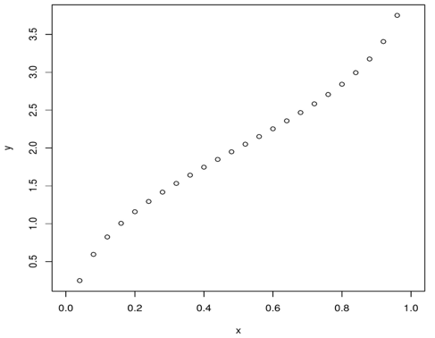
3. qnorm()
qnorm function takes the probability value and returns the cumulative value that matches the probability value.
Syntax: qnorm(p, mean, sd)
Code:
# Creating a sequence of probability values incrementing by 0.04.

x <- seq(0, 1, by = 0.04)

# mean is 2 and standard deviation as 1.

y <- qnorm(x, mean = 2, sd = 1)

# Plotting the graph.

plot(x,y)

# Saving the file.

dev.off()
Output:
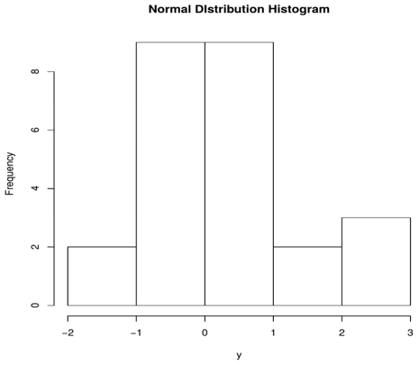
4. Rnorm()
Rnorm generates random numbers that are normally distributed. We use the random numbers and plot them on the histogram to show normally distributed numbers.
Syntax: rnorm(n, mean, sd)
mean-mean value of the data. The default value is zero. sd-standard deviation. The default value is 1. p is a set of probabilities.
Code:
# Sample of 25 numbers which are normally distributed.

y <- rnorm(25)

# Plot the histogram for this sample.

hist(y, main = "Normal DIstribution Histogram")

# Save the file.

dev.off()
Output:
Let’s now tweak the histogram by adding the color by using the simple parameter col: “color.”
Color: You Can Input Any Color. The above function can be tweaked as below to change to solid colors.
Code:
hist(y, main = "Normal Distribution Histogram",col="blue" )
Output:
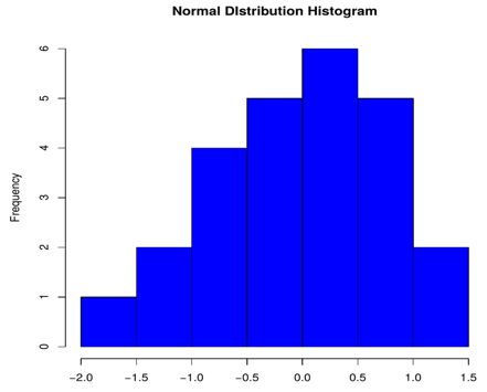
We can use the “col” parameter with any of the above four functions.
Advantages of R Normal Distribution
Given below are the advantages mentioned:
- Most of the quantities follow the normal distribution, which fits the normal phenomenon like heights, blood pressure, IQ levels.
- It makes it easy for statisticians to work with data when it is normally distributed.
- It can also be used to control the quality. The bell curve is also known as the Gaussian distribution.
Recommended Articles
This is a guide to R Normal Distribution. Here we discuss the functions and advantages of R normal distribution with plotting the graph. You can also go through our other related articles to learn more –
