Updated March 20, 2023
Introduction to Binomial Distribution in R
Binomial Distribution in R is a probability model analysis method to check the probability distribution result which has only two possible outcomes.it validates the likelihood of success for the number of occurrences of an event. It categorized as a discrete probability distribution function. There are inbuilt functions available in R language to evaluate the binomial distribution of the data set. The binomial distribution in R is good fit probability model where the outcome is dichotomous scenarios such as tossing a coin ten times and calculating the probability of success of getting head for seven times or the scenario for out of ten customers, the likelihood of six customers will buy a particular product while shopping. They are dbinom, pbinom, qbinom, rbinom.
The formatted syntax is given below:
Syntax
- dbinom(x, size,prob)
- pbinom(x, size,prob)
- qbinom(x, size,prob) or qbinom(x, size,prob , lower_tail,log_p)
- rbinom(x, size,prob)
The function has three arguments: the value x is a vector of quantiles (from 0 to n), size is the number of trails attempts, prob denotes probability for each attempt. Let’s see one by one with an example.
1. dbinom()
It is a density or distribution function. The vector values must be a whole number shouldn’t be a negative number. This function attempts to find a number of success in a no. of trials which are fixed.
A binomial distribution takes size and x values. for example, size=6, the possible x values are 0,1,2,3,4,5,6 which implies P(X=x).
n <- 6; p<- 0.6; x <- 0:n

dbinom(x,n,p)
Output:
![]()
Making probability to one
n <- 6; p<- 0.6; x <- 0:n

sum(dbinom(x,n,p))
Output:
![]()
Example 1 – Hospital database displays that the patients suffering from cancer, 65% die of it. What will be the probability that of 5 randomly chosen patients out of which 3 will recover?
Here we apply the dbinom function. The probability that 3 will recover using density distribution at all points.
n=5, p=0.65, x=3
dbinom(3, size=5, prob=0.65)
Output:
![]()
For x value 0 to 3 :
dbinom(0, size=5, prob=0.65) +

+ dbinom(1, size=5, prob=0.65) +

+ dbinom(2, size=5, prob=0.65) +

+ dbinom(3, size=5, prob=0.65)
Output:
![]()
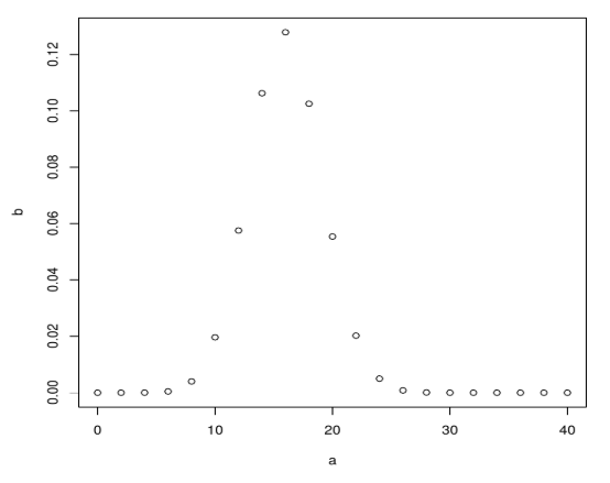
Next, create a sample of 40 papers and incrementing by 2 also creating binomial using dbinom.
a <- seq(0,40,by = 2)

b <- dbinom(a,40,0.4)

plot(a,b)
It produces the following output after executing the above code, The binomial distribution is plotted using plot() function.
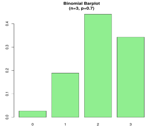
Example 2 – Consider a scenario, let’s assume a probability of a student lending a book from a library is 0.7. There are 6 students in the library, what is the probability of 3 of them lending a book?
here P (X=3)
Code:
n=3; p=.7; x=0:n; prob=dbinom(x,n,p);

barplot(prob,names.arg = x,main="Binomial Barplot\n(n=3, p=0.7)",col="lightgreen")
Below Plot shows when p > 0.5, therefore binomial distribution is positively skewed as displayed.
Output:
2. Pbinom()
calculates Cumulative probabilities of binomial or CDF (P(X<=x)).
Example 1:
x <- c(0,2,5,7,8,12,13)

pbinom(x,size=20,prob=.2)
Output:
![]()
Example 2: Dravid scores a wicket on 20% of his attempts when he bowls. If he bowls 5 times, what would be the probability that he scores 4 or lesser wicket?
The probability of success is 0.2 here and during 5 attempts we get
pbinom(4, size=5, prob=.2)
Output:
![]()
Example 3: 4% of Americans are Black. Find the probability of 2 black students when randomly selecting 6 students from a class of 100 without replacement.
When R: x = 4 R: n = 6 R: p = 0. 0 4
pbinom(4,6,0.04)
Output:-
![]()
3. qbinom()
It’s a Quantile Function and does the inverse of the cumulative probability function. The cumulative value matches with a probability value.
Example: How many tails will have a probability of 0.2 when a coin is tossed 61 times.
a <- qbinom(0.2,61,1/2)

print(a)
Output:-
![]()
4. rbinom()
It generates random numbers. Different outcomes produce different random output, used in the simulation process.
Example:-
rbinom(30,5,0.5)

rbinom(30,5,0.5)
Output:-
![]()
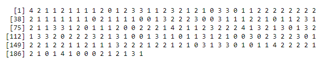
Each time when we execute it gives random results.
rbinom(200,4,0.4)
Output:-
Here we do this by assuming the outcome of 30 coin flips in a single attempt.
rbinom(30,1,0.5)
Output:-
![]()
Using barplot:
a<-rbinom(30,1,0.5)

print(a)

barplot(table(a), border=FALSE)
Output:-
To find the mean of success
output <-rbinom(10,size=60,0.3)

mean(output)
Output:-

Conclusion – Binomial Distribution in R
Hence, in this document we have discussed binomial distribution in R. We have simulated using various examples in R studio and R snippets and also described the built-in functions helps in generating binomial calculations. Therefore, a binomial distribution helps in finding probability and random search using a binomial variable.
Recommended Articles
This is a guide to Binomial distribution in R. Here we have discuss an introduction and its functions associated with Binomial distribution along with the syntax and appropriate examples. You can also go through our other suggested articles to learn more –
