Updated August 21, 2023
Pivot Table with Multiple Sheets (Table of Content)
Pivot Table with Multiple Sheets
Most of you know about pivot tables; it is a handy tool to consolidate all your data in one table and get the figures for particular things as required. Here, data could be sales reports, highest-selling products, average sales, and more.
If your data is in different workbooks or worksheets, you have two ways to get a pivot table from it; the first one gets all the data in a single sheet by copy-paste and then make a pivot table from it; another one is to use this feature of MS Excel wizard to make a pivot table from multiple sheets.
How to Create Pivot Table from Multiple Sheets in Excel?
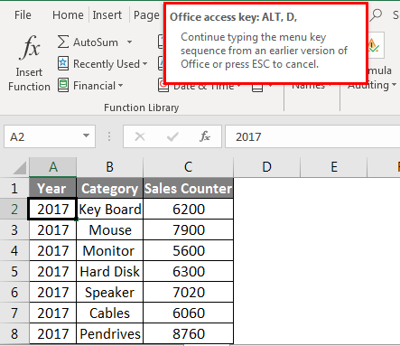
For instance, let’s assume we have data from a shop selling computer parts, like Keyboard, Mouse, Hard disk, Monitor, etc. They have this data on a yearly basis; as shown in the image below, we are taking three years of data with only three columns which one is using to identify the particular sheet.
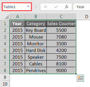
The above data are in a single workbook and multiple sheets; we have given the name of the sheet respectively to the sales year.
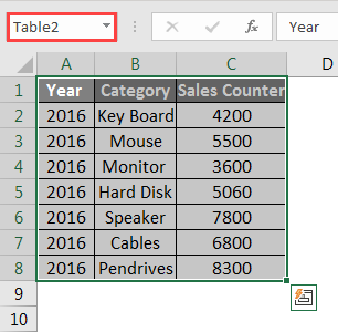
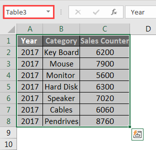
We have data for 2015, 2016 & 2017 and ensure the given data have identical columns, categories, and sales counters.
Here the data shows the product sold by this shop in the respective years.
To create the master pivot table from these different worksheets, we need to enter into the Pivot table and Pivot Chart Wizard; this function was disabled in earlier MS Office versions, but we can access the same by the shortcut keys Alt + D + P.
Creating a Pivot Table with Multiple Sheets
- Alt + D is the access key for MS Excel, and after that, by pressing P after that, we’ll enter the Pivot table and Pivot Chart Wizard.
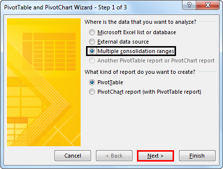
- We can see the Pivot table and Pivot Chart Wizard – Step 1 of 3 as shown below.

- Here wizard will ask you two questions we need to answer, the same as follows.
Where is the data that you want to analyze?
- There are four options; we will select option no. 3 – Multiple Consolidation Ranges
What kind of report do you want to create?
Here we’ll have two options; we will select option no. 1 – Pivot Table
Now clicn “Next,” and you’ll see Step – 2a of 3, as shown below.
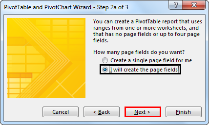
As per the above image, it asks you, “How many page fields do you want?” Here we will create the Page fields, so select “I Will Create the Page Fields,” then clicn “Next.”
You’ll see Step – 2b of 3 below the image.

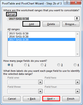
As per the above image, we now have to select the ranges for our Pivot table,
- Select the entire table (Range) from our first sheet, “2015”, and then click “Add.“
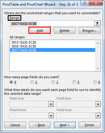
Now select the table from sheet “2016” and then click “Add” Similarly, add the range of our table from sheet “2017”, As we can see, All ranges we have selected from our different worksheets, and here the wizard has the option of “How many page field do you want?“, by default, it remains zero. Still, we have to select 1, as we want our table to be differentiated by one field (Year); here, we have selected a 1-page field to provide the name for that particular field by selecting the ranges. So we will give the field’s name in that table, which is 2015, 2016, and 2017 as per the image below.
- Now by clicking Next, we can see the dialog box of step 3 of 3 as shown below:
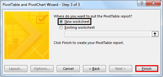
As per the above image, the wizard allows you to put the Pivot table in a net oe existing worksheet.
- Here we want our table in a new worksheet, so select that option and click Finish. Now we have a Pivot table on the 4th sheet in our workbook. Let’s look into the below screenshot for your reference.
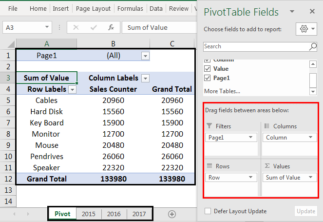
- As per the above image, we can see that another sheet has been added; we will rename the same as Pivot, So now the pivot table is ready.
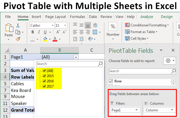
- By default, the pivot shows the entire data with all these three sheets (2015, 2016 & 2017) included.
- The pivot table is provided with the filters; we can select the filters in the column we want.
- But here, by default filter is provided for the category and the year of sales; during step 2b, we have selected one-page fields as 2015, 2016, and 2017; we can see them in the filter section mentioned all as per shown in the below image, we can select the data accordingly.
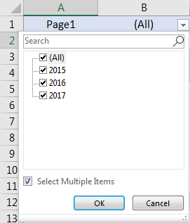
- As per the below image, we can also filter the category and see the entire data of that category sold by these three years,
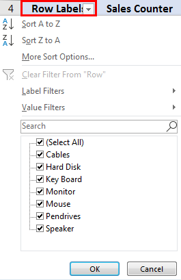
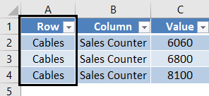
- If you want a sales counter of a particular category, you can select it from the filter provided in the category else; if you want a separate sheet for that particular category, double-click on it, and the data of that category will be shown in a new datasheet as shown in the image below.
- For example, here we have selected cables, and we will have a separate new sheet for the cables data,
- As per the image below, the sheet shows the entire data regarding that category available in our Pivot table.
Things to Remember
- While creating the pivot table from the multiple sheets, you must remember that the sheets you want to include in the pivot table must have an identical column.
- Here, you can also give the names to the table (same as we have provided the name to the matrix), so whenever you change the data in the sheet, the same will also change in the pivot table.
Recommended Articles
This has been a guide to Pivot Table with Multiple Sheets. Here we have discussed How to create Pivot Table from Multiple Sheets in Excel, along with various steps and a downloadable Excel template. You may also look at the following articles to learn more –
