Updated June 6, 2023
Introduction to COLUMNS Formula
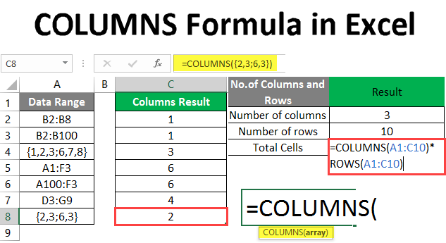
The COLUMNS Formula in Excel determines the number of columns available in the given array or the reference in the input array. It is an in-built function that comes under the Lookup and Reference function. It helps look for the number of columns in the array.
As an example, let’s assume there is an array “B2:F7”; then, in the COLUMNS function (=COLUMNS (B2:F7)) will return 5. It means 5 columns exist in the range of B2 to F7.
Syntax
COLUMNS () will return the total number of columns in the given input. There is only one argument – array.
How to Use COLUMNS Formula in Excel? COLUMNS Formula in Excel is very simple and easy. The Argument in the COLUMNS Function:
- array: It is a mandatory parameter for which the user wants to count the number of columns in the cell range.
Let’s understand how to use the COLUMNS Formula in Excel with some examples.
Example #1- How to use the COLUMNS Function in Excel
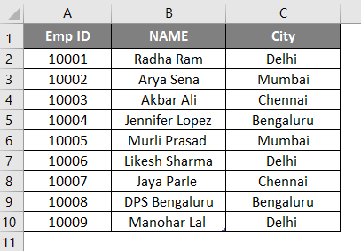
Some data is given in a table in Sheet 1, so a user wants to count the number of columns in the table.
Let’s see how the COLUMNS Function can solve this problem.
Open MS Excel; go to Sheet1, where the user wants to find out the numbers of columns in the table.
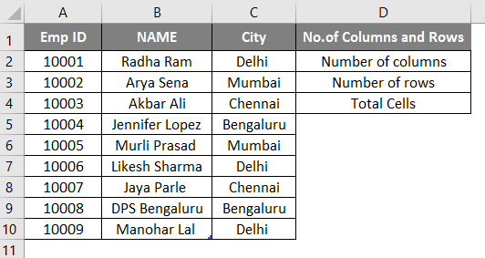
Create one header for the COLUMNS results to show the function result in column D.
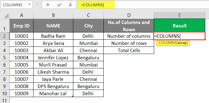
Click on cell D2 and apply the COLUMNS Formula.
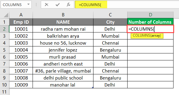
Now it will ask for an array in which the table’s range means total cells.
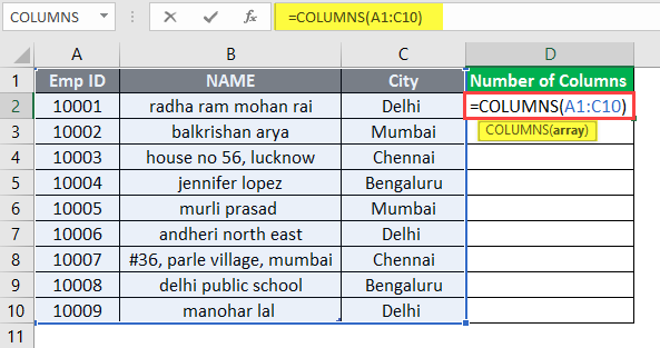
Press the Enter Key.
Now merge cells from D2 to D10.
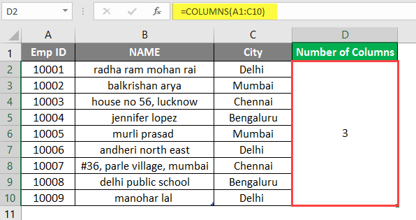
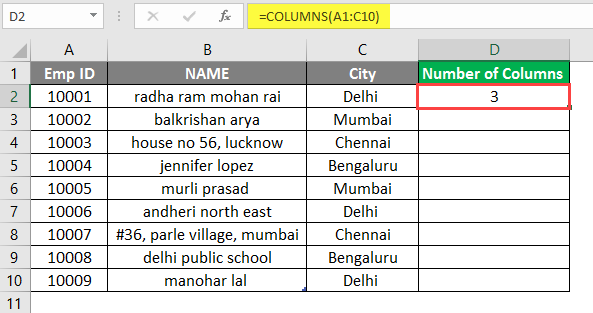
Summary of Example 1:
The user wants to find out the number of columns in the table. The function result is available in column D, which is coming as 3, which means there are a total of 3 number columns in the range A1 to C10.
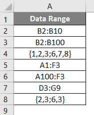
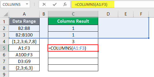
Example #2- Different Types of Arrays and References
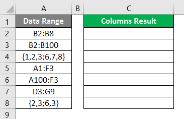
If a user wants to count the number of columns in a given data range within a table on Sheet2.
Let’s see how the COLUMNS Function can solve this problem.
Open MS Excel; go to Sheet2, where the user wants to find out the number of columns in the range.
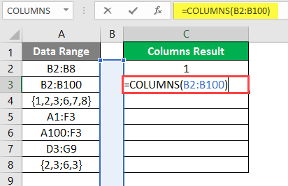
Create one header for the COLUMNS results to show the function result in column C.
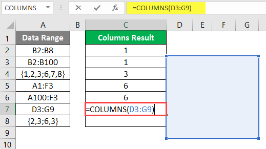
Click on cell C2 and apply the COLUMNS Formula.
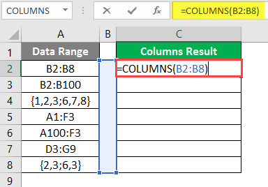
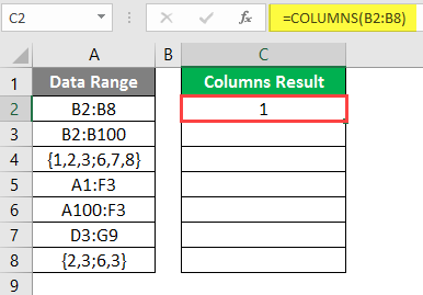
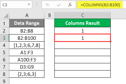
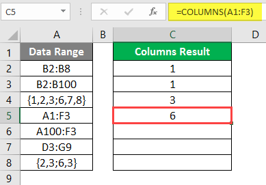
The result is shown below after using the above Formula.
Use the Columns Formula in the next cell.
The result is shown below after using the above Formula.
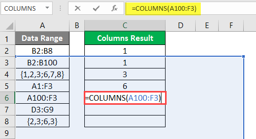
Use the Columns Formula in the next cell.
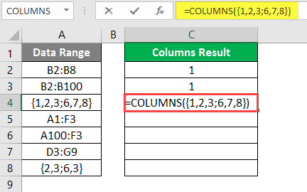
The result is shown below after using this Formula.
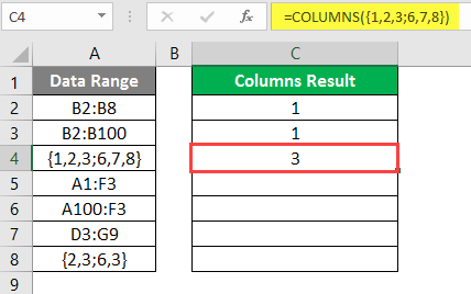
Use the Columns Formula in the next cell.
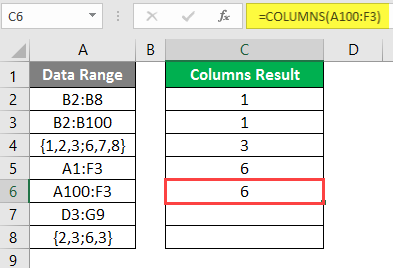
The result is shown below after using the above Formula.
Use the Columns Formula in the next cell.
The result is shown below after using this Formula.
Use the Columns Formula in the next cell.
The result is shown below after using the columns formula.
Use the Columns Formula in the next cell.
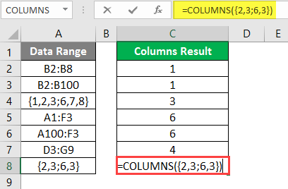
The result is shown below after using the columns formula.
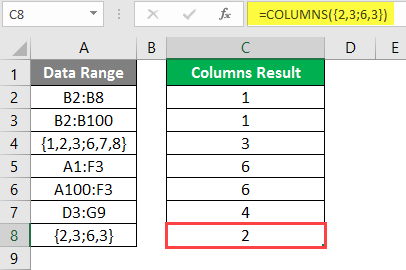
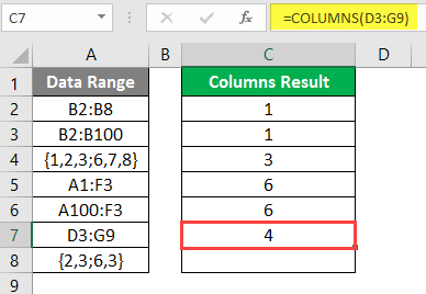
Summary of Example 2:
The user wants to determine the number of columns in the table. The function result is available in column C, which is coming for each data.
Example #3- Find the Total Cells in the Array or References
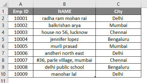
Sheet 3 contains a table with data, including Employee ID, Name, and City. So, a user wants to count the number of cells in the table.
Let’s see how the COLUMNS Function can solve this problem with the rows function.
Open MS Excel; go to Sheet 3, where the user wants to find the table’s total cells.
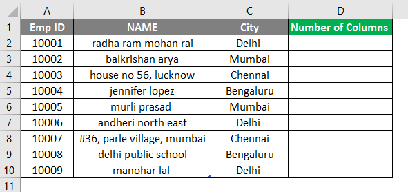
Create three headers for the COLUMNS result and rows result, and show the total cells to show the function result in column D.
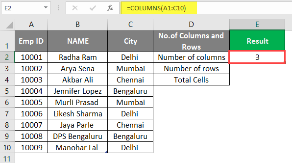
Click on cell E2 and apply the COLUMNS Formula.
It will then ask for an array in which the table’s range means the total cells, select cells A1 to C10.
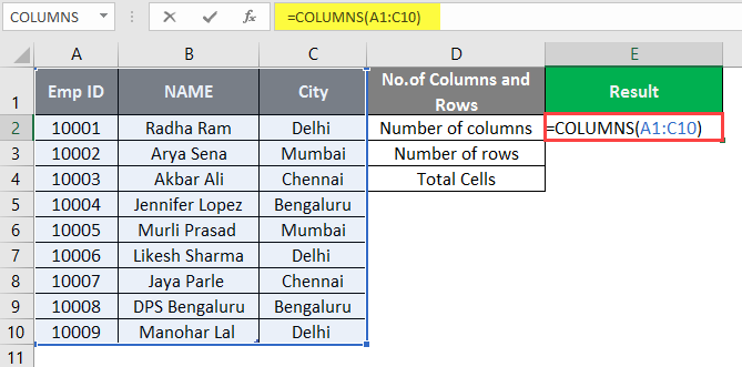
Press the Enter Key.
Click on cell E3 and apply the ROWS Function to count the total number of rows in the table.
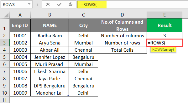
It will then ask for an array in which the table’s range means the total cells in the table, select cells A1 to C10.
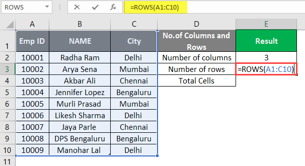
Press the Enter Key.
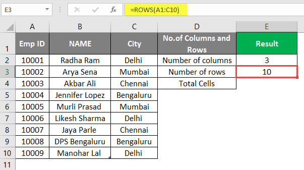
Now just multiply the cells data of the total number of columns and the total number of rows in the E4 to find out the total number of cells in the table.

‘OR’
Calculate the total number of columns and the total number of rows in cell E4 and multiply there only.
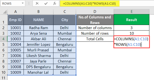
Press the Enter Key.
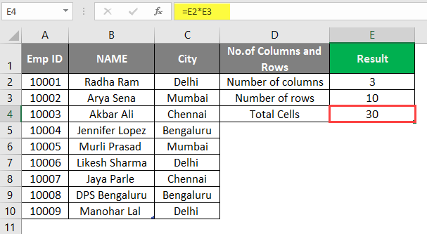
Summary of Example 3:
The user wants to find out the total number of cells in the table. The function result is available in cell F4, which comes 30 after calculation.
Things to Remember
- The COLUMNS function will return the number of columns available in the given array or the reference in the input array.
- When a user wants to determine the total number of columns present in an array, the array argument can be utilized within the Formula.
- The array argument permits the inclusion of a single cell or a reference to a single cell within the array. But it will not support multiple cells or references in the columns function; a user can pass a single range at a time.
Recommended Articles
This has been a guide to the COLUMNS Formula in Excel. Here we discuss How to use COLUMNS Formula in Excel, practical examples, and a downloadable Excel template. You can also go through our other suggested articles –
