Updated May 30, 2023
Pivot Table Count Unique (Table of Contents)
Introduction to Pivot Table Count Unique
A pivot table is the best feature that Excel includes. It takes rows into consideration and then allows us to summarize the data based on either sum or count or average or any other numerical aspect of the data we want. The best part, it also helps us counting the text values. By far, the count function within the pivot table is quite of use and needed every now and then by analysts. However, when we are in need to count unique values, there is no default function under Excel. With some tweak and twist, we can count the unique values in the Excel pivot table.
What is Count Unique?
Suppose you are running a business and have sold hose pumps to different countries in the past 12 months. Now, you want to check how many unique customers (in our example, consider the country as a customer) you have achieved during this period. The chances are that we have traded with multiple countries, and out of which, we only want to figure out the unique country values.
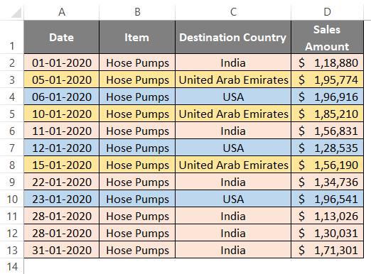
Just a small example for your reference here. We are not using the entire year’s data. Since it is a day-wise trade, it will be a huge one. Just for a realization, see the image below:
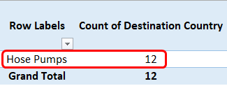
If we go through the data, we can say that there are three unique country values: India, United Arab Emirates, and the USA. However, if we do a pivot table and count the Destination Country, then the results are somewhat weird, as shown in the screenshot below:
You can see that the count for countries we traded is 12 in the pivot table, which is not a unique count. We need to amend the pivot table to get the unique count. In this article, we will make you walk through the method using which we can count the unique values in the Pivot Table. Just follow the steps below:
Before we proceed further, let me clear a thing for you. This technique of getting unique values in the pivot table applies to Excel’s 2013 or later version.
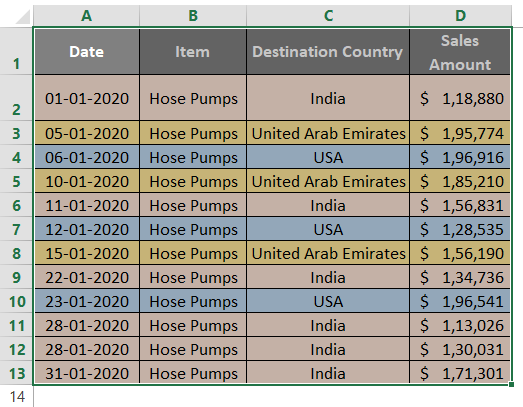
Let us only consider the data shown in the above screenshot, which is spread across A1:D13.
Step 1: Select the data range for this entire tabular data that spreads across A1 to D13.
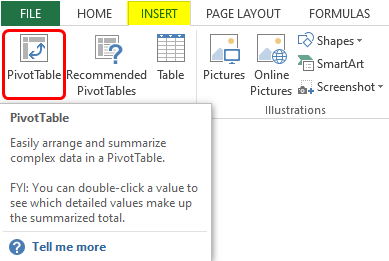
Step 2: Now, we will add a pivot table for a selected range of data. For that, go to the Insert tab placed on the upper ribbon in the Excel sheet. Click on the Insert menu tab.
Step 3: Once you click on the Insert menu tab, you’ll see different insert options associated with the selected range of cells; out of those, under the Tables group, you can see PivotTable. Click on it to add a pivot table for a given range of data.
You have a shortcut to add a pivot table. You can use Alt + N + V as a keyboard shortcut to insert a pivot table. This will also allow you to add a pivot table in Excel using the keyboard shortcut.
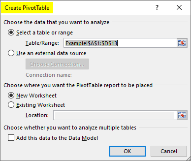
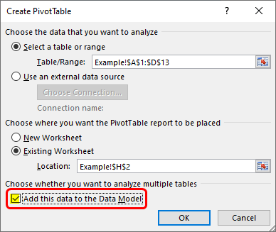
Step 4: As soon as you click on the PivotTable option under the Tables group inside the Insert tab, a new window will pop up named Create PivotTable, as shown in the image below:
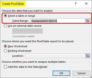
Step 5: Within the Create PivotTable window that pops up, you can add the range of cells on which you need to apply the pivot table. This can be done under the Select a Table or range section. By default, our range of data has been selected at the start of the creation itself.
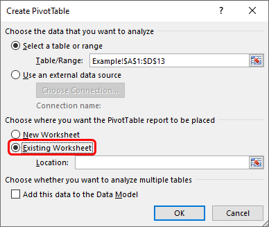
Step 6: Destination, where the pivot table needs to be created, has two choices. Either you can create it on a new worksheet or the existing worksheet. Click on the radio button next to it. We will choose the Existing Worksheet option.
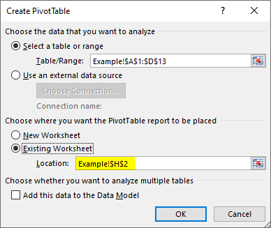
Step 7: Give the location cell where you want to store the pivot table in the existing worksheet. I will use the location as cell H2.
Step 8: At the bottom of the Create PivotTable window, you’ll see a checkbox Add this data to the Data Model. You need to tick select this checkbox. This will allow us to count the unique values in the pivot table.
Click on the OK button, and that’s it. We will have a blank pivot table, as shown in the screenshot below:
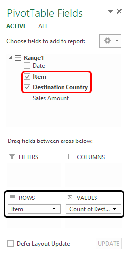
Step 9: Under Pivot Table Fields, select Item under Rows and Destination Country under the Values section below. You can do this by dragging and dropping fields with the mentioned name under the respective tabular section.
We are still not getting a unique Destination Country count as expected. To get the same, follow the step below:
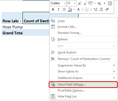
Step 10: Right-click on the Count of Destination Country Column, and you will see a list of options as shown below. Select the Value Field Settings… option out of those.
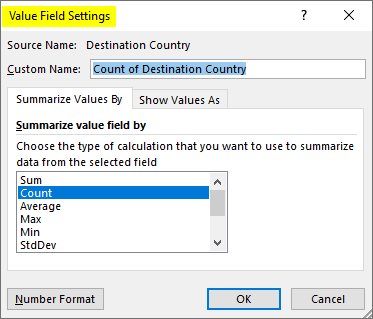
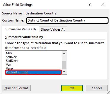
This will open up the Value Field Settings window, as shown below. We clearly could see that the current summarization type is COUNT for value fields (i.e., Destination Country column). Since the COUNT option only counts the number of rows present in source data, in our case, it is answering 12 because we have 12 rows in the given data for Destination Country.
However, it should not be like this; we need unique distinct values to be counted for the Destination Country column. To achieve this, you need to do something.
Navigate through the Summarization type using the scroll bar and click select the Distinct Count option to count the unique values. Click on the OK button once done.
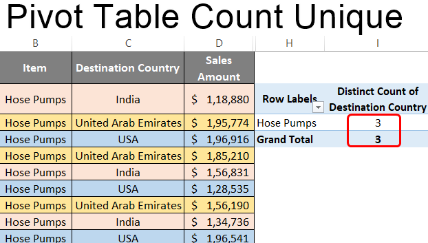
As soon as you select the Distinct Count and hit the OK button, you’ll get the value for the count of the Destination Country column, as shown in the screenshot below. It specifies the unique count of values present under the Destination Country column.
This is how we can get the count of unique values under PivotTable in Excel. We will end this article here. We have some points to be remembered for the same.
Things to Remember in Pivot Table Count Unique
- The method used in this example is working on Excel’s 2013 and later versions. For previous versions of Excel, you might need to use different techniques, such as Pivot of Pivot Table, etc., to get the unique count (This is out of the scope of this article).
- There is no default way to capture Excel’s unique count of values. You need to use the Add this data to the Data Model option at the bottom of the Create PivotTable window.
Recommended Articles
This has been a guide to Pivot Table Count Unique. Here we discuss How to use Pivot Table Count Unique, practical examples, and a downloadable Excel template. You can also go through our other suggested articles –
